REVIEW: Electron Tomography of Biological Samples
S. Marco*, T. Boudier, C. Messaoudi, and J.-L. Rigaud
Institut Curie, Section Recherche, UMR-CNRS 168 et LRC-CEA 34V 11, rue Pierre et Marie Curie, 75005 Paris, France; fax: +33 1 40 51 36 06; E-mail: sergio.marco@curie.fr* To whom correspondence should be addressed.
Received July 23, 2004
Electron tomography allows computing three-dimensional (3D) reconstructions of objects from their projections recorded at several angles. Combined with transmission electron microscopy, electron tomography has contributed greatly to the understanding of subcellular structures and organelles. Performed on frozen-hydrated samples, electron tomography has yielded useful information about complex biological structures. Combined with energy filtered transmission electron microscopy (EFTEM) it can be used to analyze the spatial distribution of chemical elements in biological or material sciences samples. In the present review, we present an overview of the requirements, applications, and perspectives of electron tomography in structural biology.
KEY WORDS: electron microscopy, electron tomography, image analysis, 3D-reconstruction
Methods for elucidating three-dimensional (3D) structures of subcellular components constitute one of the largest assets of modern biology because they allow understanding of structure-function relationships at the molecular level. Structural analysis by X-ray diffraction and nuclear magnetic resonance (NMR) has brought considerable structural information on individual proteins and small protein complexes. However, cellular machines, made up of multiple complex components, remain inaccessible to these structural techniques. During the last half of the XX century, the developments of microelectronics and data processing have made transmission electron microscopy (TEM) a powerful tool for the study of those cellular machines too complex to be analyzed by X-ray or NMR. Indeed, the resolution of three-dimensional reconstructions is increasing thanks to the design of new electron microscopes presenting a more coherent beam (field emission gun microscopes) equipped with digital recording systems. Moreover, the increase in the storage and computing powers of the data-processing equipment made possible the processing of a greater amount of data as well as the application of powerful algorithms for image analysis and 3D-reconstruction. In parallel, the techniques for sample preparation for TEM have also evolved. Thus, methods that allow observing samples in vitreous ice (cryo-microscopy) avoid the artifacts of negative staining and allow a better safeguarding of the biological material by removing the effects of dehydration [1-3]. All these technical and methodological developments have made it possible to achieve 3D-reconstructions of macromolecular complexes by TEM (single particle analysis) at resolutions allowing fitting to X-ray or NMR structures [4, 5]. It is then possible to analyze the interactions that stabilize the macro-complexes and to look further into the comprehension of their structure. In this context, another asset of TEM combined with the digital analysis of images is to study conformational changes of protein or macromolecular complexes without passing by the limiting step of crystallization. Indeed, with TEM it is possible to directly observe individual proteins and complexes in solution in different conformational states induced by substrates, effectors, or inhibitors. TEM thus evolved from morphological description to the study of dynamic processes.
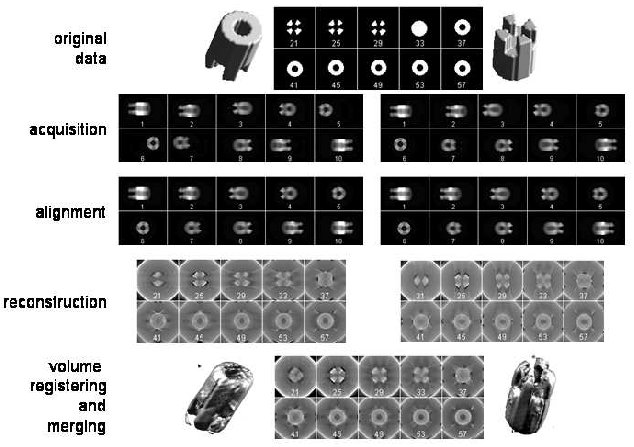
In the last 20 years, following the automation of the image recording process under the microscope, a new 3D approach has been born: electron tomography [6, 7]. Electron tomography is based on the acquisition of a small number of projections (100-200) from an individual object. These projections are aligned and combined, to generate a three-dimensional reconstruction of the original object. A standard tomographic reconstruction process is constituted of the steps detailed in Fig. 1. At least two types of software are required to perform electron tomography: software for automatic recording of images at different tilt angles on the electron microscope and software for image analysis to reconstruct and analyze the volumes.
Electron tomography gives access to structural information at subcellular organization levels. Thus, volumes of mesoscopic objects (size between 0.1 and 1.0 µm) can be computed and analyzed [8-12]. Since electron tomography is based on the recording of projections of a single object oriented at different angles in space, the reconstruction process implies the determination for each projection of its relative orientation and the combination of all the projections to recover the original object [12]. This approach has made it possible to obtain 3D information on cellular structures like kinetocores [13], Golgi apparatus [14], mitochondria [15], and basal bodies [16] with microscopes operating at high voltage (1 MV). Other structures have been solved using standard microscopes (voltage <=300 kV, LaB6, or field-emission gun cathodes) such as chitin secretion organelles [17], bacteriophages [18], chromosomes [19], or centrosomes [20, 21].Fig. 1. Different steps required for electron tomography and effects of the missing wedge. The left panel in the “acquisition” step shows some of the projections obtained between -60 and +60° of the object shown in the original data (top). These projections have been calculated to simulate drift during acquisition. The projections are then centered as shown in the left panel of the “alignment” step before computing a 3D-reconstruction. The left panel in the “reconstruction” step shows ten sections of the computed volume. The effects of the missing wedge are evidenced by the loss of information observed when planes are compared with the original data (top). To compensate for the missing wedge, a second set of projections can be generated by rotating 90° the volume in the horizontal plane, as shown in the right panel of the “acquisition” step. These projections are centered (right alignment panel) and a 3D-reconstruction calculated (right reconstruction panel). The missing wedge present in the reconstruction computed from the data set in right panels is perpendicular to the one observed in the volume calculated from the data set on the left panel. The combination of the two volumes (double axis tomography) reduces the missing wedge effects as shown in the “volume registering and merging” raw resulting in a 3D-reconstruction similar to the original data. Numbers in images correspond to the projections or sections numbers.
SAMPLE PREPARATION
The first requirement in performing electron tomography is to prepare samples. Several possibilities exist depending on the type of information to be recovered. Proteins or macromolecular complexes can be prepared from solutions by negative staining [22], fast-freezing [3], or cryo-negative staining [2]. In the case of cellular samples, due to their thickness, it is necessary to obtain sections after chemical fixation and embedding in plastic resins. However, such preparations damage the biological ultrastructure of the samples [23]. Thus, high-pressure freezing [24] and cryo-fixation [9] are currently used to get better sample preservation.
Negative staining is based on the use of heavy metal salts, such as uranyl acetate, ammonium molybdate or phosphotungstic acid, which surround the samples and are visualized as electron dense surfaces under the microscope. This method provides rapid information about the structural shape and organization of molecules. However, samples are dehydrated and flattened, reducing the final quality and resolution of the reconstructed volumes. In order to increase the resolution of the reconstructed volumes, great efforts are currently under development, such as rapid freezing in liquid ethane, which preserves the structure of the samples [25]. However, images recorded on frozen-hydrated samples present low contrast and high sensitivity to radiation. A promising technique, which reduces the drawbacks of freezing in liquid ethane, is cryo-negative staining. This approach combines negative staining with freezing in liquid ethane under hydrated conditions, resulting in an increase in the contrast of the images while the samples remain hydrated and protected against radiation [1].
For cellular samples, classic preparation methods require chemical fixation and embedding in plastic resins. However, this approach generates artifacts that can be reduced by using physical fixation under high-pressure conditions [9, 26]. Moreover, the recent development of cellular sample preparation allows freezing samples directly [27] and getting sections that can be observed on the microscope without any staining agent (cryo-sections). This approach preserves the sample under nearly native conditions. However, a limitation of this preparation method is the requirement of highly specialized equipment, such as cryo-ultramicrotomes with special cryo-knifes for sectioning [28] or energy filters for contrast enhancement of the images.
PRINCIPLES AND PROBLEMS OF IMAGE RECORDING IN ELECTRON
TOMOGRAPHY
Concerning the image acquisition under the electron microscope, three main problems should be noted [7]: radiation damage, mechanical drift, and focus variations. Radiation damage [29] is probably the main problem in electron tomography, because the recording of a single tomographic series implies taking at least 100 images (for projection angles from -50 to +50°, each degree) of the same area. In practice, biological samples embedded in plastic resins can lose up to 30% of their thickness [30] during the acquisition and frozen hydrated samples can be destroyed by the electron beam. Radiation damage limits the magnification used on the microscope and then reduces the resolution of tomographic reconstructions. To prevent radiation damage, two procedures can be considered: reduction of the number of electrons required to record one image or protection of the sample from the effects of radiation. In the first approach, the use of field-emission gun microscopes, with electron beams more coherent and brilliant than those generated by standard LaB6 microscopes, as well as the use of slow-scan CCDs presenting high sensitivity to electrons are current solutions [31]. Concerning the protection against radiation, samples embedded in plastic resins can be slowly frozen in liquid nitrogen, then transferred to the electron microscope at -168°C, and observed at this temperature. Our preliminary tests performed on semi-thin samples (200 nm thick) indicated that the thinning phenomenon is reduced to less than 10%.
The drift phenomenon can be observed during acquisition as the tilt angle is changed. This mechanical drift, if coupled to the thermal drift in the case of samples observed at liquid nitrogen temperature, can induce an irreversible loss of data. A simple approach to minimize the drift effect is to use cross-correlation functions to calculate the displacements between two consecutive images recorded at different angles, and then re-center the sample projection before taking again a new image at the current angle (Fig. 2a). This method is precise but requires two acquisitions per angle that increase the irradiation of the sample. Thus, it can be used only for samples rather resistant to irradiation. A second approach consists in estimating the drift that corresponds to the two preceding angles and then in applying a correction of this drift before recording the image at the current angle (Fig. 2b). This method presents the advantage that sample is not additionally irradiated [32]. A third approach consists in performing a pre-calibration of the microscope by calculating and storing the drift modifications existing between consecutive angles. The stored drift correction values are then applied during the real acquisition of the series [33]. Recent algorithms can predict image displacement based on the assumption that the sample follows a simple rotation. As a consequence, it is not necessary to either record additional images for tracking and focusing during the course of data collections or to spend time in a lengthy pre-calibration of stage motions [34, 35].
Concerning focus variations, they are negligible if the tilt-axis is aligned with the eucentric axis. In practice, this alignment is never perfect and focus variations become an important factor that could reduce the quality of the final reconstructions, especially with thick specimens (thickness > 300 nm) such as used for tomography. To prevent this problem, autofocus programs based on the comparison of Fourier transform from images are currently implemented in all existing software for tomographic acquisition [33].Fig. 2. Drift correction methods during acquisition. a) Precise drift estimation. The shift computed by cross-correlation between images recorded at angles n - 1 and n is applied before acquiring a final projection at angle n. b) The shift estimated between images recorded at angles n - 2 and n - 1 is applied before acquiring the projection at angle n.
THREE-DIMENSIONAL RECONSTRUCTION ALGORITHMS
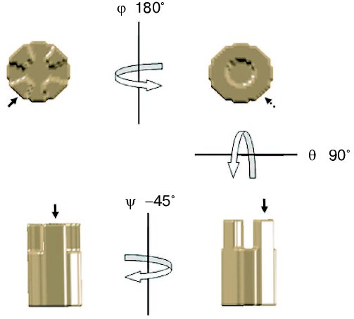
Once the tilted series have been acquired, the 3D-reconstruction can be computed from the raw data. The reconstruction process implies the determination, for each projection, of the orientation in space of the object being at its origin. Considering that this position is defined by the Euler angles (phi. horizontal rotation; theta, vertical rotation; and iota, the second horizontal rotation following the application of phi and theta), reconstruction algorithms consist in determining the Euler angles for each projection before merging them (Fig. 3, see color insert) [12]. However, before determining these angles it is important to shift the images to a common center and to cut the region of interest common to the whole image set. This post-acquisition centering preliminary step is required because the procedures for drift correction during acquisition are not able to compensate it totally. The centering process is done by fixing the position of a reference image and shifting a second one to different (X, Y) positions. Then, for each (X, Y) position, the cross-correlation coefficient, which measures the similarity between the two images, is calculated and the second image is displaced to the (X, Y) coordinates that maximize the value of the cross-correlation coefficient. Once the image set is centered, the Euler angles can be calculated. In the case of cellular tomography, it is simple because a single object has been tilted around a single axis, so there is no horizontal rotation (phi = 0). The tilt angle (theta) is known for each image from the microscope, and if images are rotated (different iota_values) each rotation angle can be computed by a rotational cross-correlation. In practice, differences in the iota value are negligible. In the case of single particle analysis, the approach to calculate the angles is slightly different. The geometrical relationships existing between several projections of a homogeneous biochemical sample have to be computed, which implies the calculation of the Euler angles for each object. For this purpose, iterative reference-free alignment algorithms are used [36, 37].
Once the Euler angles have been determined, it is possible to compute the three-dimensional reconstruction from the set of projections. The most frequently used algorithm to reconstruct volumes from projections is the weighted back-projection [38]. This algorithm is based on the central section theorem which states that the 2D Fourier transform of a projection through a 3D volume will coincide with a plane passing through the origin of the 3D Fourier transform of the volume with the same orientation as the projection. Thus, the Fourier transform of each image can be calculated and placed in the 3D Fourier space based on the computed Euler angles. When all the Fourier transforms are placed in the 3D Fourier space, a 3D Fourier transform is generated. The inverse of this 3D Fourier transform corresponds to the original object volume. The original data set should contain all the possible orientations of the object to calculate an exact reconstruction. Nevertheless, the ideal case, in which the Fourier space is completely filled from the projections, does not occur in electron tomography since it is not possible to tilt the sample at 90° inside the electron microscope. Actually, the effective sample thickness to be crossed by the electrons is equal to the original thickness divided by the cosine of the tilt angle (theta). Thus, when theta = 90° the sample thickness becomes infinite, meaning that no image can be recorded. In practice, angle values between -60 and +60° (sometimes 70°) are used. This limitation in the maximum tilt angle that can be used to record images induces a missing of data in the Fourier space known as the missing wedge [39]. To reduce the effect of the missing wedge, it is possible to record several tomographic tilt series of a single object after rotation in the horizontal plane. This approach, known as multiple axis tomography, allows reducing the missing wedge to a missing cone (Fig. 1). An additional problem related to the relationship between the sample thickness to be crossed by the electron beam during acquisition and the tilt angle (theta) is that the number of electrons arriving to the ssCCDs decrease with the absolute value of the tilt angle. This implies that the images become darker while the tilt angle increases. To reduce this effect, it is possible to consider that the average luminosity of the images decrease with the increment of the tilt angle. Thus, the exposure time for each image should be increased by a factor equal to the starting time defined at theta = 0° divided by the cosine of the tilt angle (theta) at which the image is recorded.Fig. 3. Use of Euler angles. To get a lateral view horizontally rotated by 45° (bottom left) from a front view (top left) of a volume (phi = 0, theta = 0, iota = 0), it should be rotated horizontally (phi_= 180°, theta = 0, iota = 0) giving a back view (top right), then vertically (phi = 180°, theta = 90°, iota = 0) as shown at bottom right and finally rotated again by 45° on the horizontal plane (phi = 180°, theta = 90°, iota = 45°). Arrow shows the position of a relevant feature of the volume.
IMPROVING TOMOGRAM RESOLUTION
Measuring the quality of the 3D-reconstructions is still an open problem and several methods have been proposed to calculate the resolution of volumes [40-43]. Most of them require the calculation of two independent reconstructions, which implies the division of the original data set into two sub-sets. This represents a drawback for tomography because of the few recorded projections number. To solve this limitation, a new approach based on the signal-to-noise ratio, already used for single particle analysis [44], has been recently proposed for tomograms. This approach measures the consistency between the projections calculated from the reconstructed volume and the original data set [45, 46]. The algorithms for computing volume resolution, as well as those required to perform reconstructions and models from tomographic series, have been implemented in public software facilities (table). However, the development of algorithms for multiple axis tomography to improve resolution is a recent topic. Multiple axis tomography requires the combination of several volumes of a single object, which results in an increment of the signal-to-noise ratio of the final reconstruction as well as in the reduction of the missing wedge. To merge volumes, it is necessary to compute the 3D rotational and translational shifts existing between the volumes. A possible approach is to calculate the projections of each volume and cross-correlate them to compute the phi angles as well as the shifts. The shift and angle corrections are applied to the volumes, bringing them to a common center in space, before computing an averaged volume. To refine the shifts and phi values and to determine theta_and iota, reference-free alignment algorithms, used for single particle approaches [36, 37], can be adapted in 3D. This approach has been successfully tested in the case of ribosomes, leading to a significant resolution improvement [47].
Public software facilities for electron tomography
Another approach to improve resolution is to combine volumes from different objects belonging to a single morphological group. In this case, the combination of tomograms requires classification before averaging since sample heterogeneity may induce a loss of details. Volumes classification can be efficiently done by using self-organizing neural networks [48, 49]. For instance, Pascual-Montano et al. [50] have applied this method to reconstruct the insect flight muscle.
Finally, other possibility for resolution improvement is to combine cellular tomography and single particle analysis [32]. This approach can only be applied to objects that can be obtained in several copies such as proteins, viruses (including multi-symmetrical virus like T4-bacteriophages), or organelles like centrioles. This method consists of two steps: first a reconstruction of a reference volume by cellular tomography, and second, the determination of the final 3D-reconstruction from frozen-hydrated samples. The computation of the reference volume implies performing independent 3D reconstructions of single objects by cellular tomography and combining them. The objects used to for the reconstructions of the reference volume can be prepared using any of the methods described in the sample preparation section. Then, all the projections of the volume are computed for all possible orientations. This first step is followed by the comparison between the untilted images, recorded from frozen hydrated samples, and the projections of the reference volume to compute the Euler angles of each image. Moreover, procedures for information recovery such as contrast transfer function (CTF) correction [51, 52] can be used on untilted images leading to a significant resolution improvement. Once the shifts and Euler angles are determined and the CTF is corrected, the experimental projections from the frozen hydrated samples are combined to build up the final 3D-reconstruction. This approach presents the advantage that large and complex objects not analyzable by other structural methods can be resolved at nanometric resolutions [32]. In addition, the use of frozen hydrated samples, irradiated only once with a low electron dose (less than 10 e- per 1 Å2), minimizes the deformation of the structures and facilitate the comparison of the reconstruction with data coming from X-ray crystallography.
NEW DEVELOPMENTS IN ELECTRON TOMOGRAPHY
Future developments in molecular and cellular tomography will focus on new image processing methods. In particular, it will be important to develop algorithms in order to register volumes calculated by several structural analysis methods at different resolution values. It is already possible to fit macromolecular volumes of complexes in 3D-reconstructions of cellular mesoscopic structures [53, 54] such as X-ray or NMR data of individual components can be fitted in volumes obtained by TEM from macro-complexes. To fit X-ray data into volumes of molecules computed by single particle analysis, public software, such as Situs [55] or URO [56], is accessible over the Internet. Volumes computed from a crystallographic data set are filtered at the same resolution than those calculated from microscopy and registered by cross-correlation. A similar approach exists for the fitting of 3D-reconstructions from single particle analysis into cellular tomography data. These approaches allow a better understanding of the molecular organisation of cells. However, all the sample preparation methods for electron tomography impose specimen fixation, which constitute a major problem to study any living cells. A possible solution to overcome this drawback is to combine electron and confocal microscopy by using, for instance, samples combining a fluorescent dye with a dense marker, like Fluoro-Nanogold (FNG) [57, 58].
In the context of combining different structural approaches, it is also possible to perform multidimensional analysis by coupling electron tomography and energy filter transmission electron microscopy (EFTEM). This new EFTET (energy filter transmission electron tomography) structural approach allows studying the 3D distribution of chemical elements in inorganic and organic materials. Relevant information has been obtained in the study of interfaces in material sciences [59, 60] as well as in the analysis of iron distribution in magnetotactic bacteria [61]. However, no public software to compute 3D chemical maps from EFTET images are available, which limits the use of EFTET to laboratories having experience in electron microscopy and software development. Nevertheless, important efforts are currently being made to develop public software for EFTET, and a preliminary multi-platform program is already available (table). Finally, the use of energy loss filters allows the observation of samples presenting thickness close to 800 nm [39], which constitutes an alternative to the combination of volumes computed from serial sections to calculate the 3D-structure of entire subcellular structures [62].
In conclusion, tomography combined with digital image analysis is becoming a powerful structural technique, which allows studying objects from molecules to subcellular organelles and cells. However, the computation of tomograms at the best possible resolution is not the final step for electron tomography. The complexity of the data existing in the reconstructions requires the development and use of rendering software, which includes volume segmentation and denoising. Important efforts are being made to develop algorithms for automatic segmentation of volumes [63], since segmentation is presently performed manually. Regarding denoising, a new generation of algorithms is successfully applied to electron tomograms facilitating the interpretation of complex structures [64-66].
The authors thank the French INSU GEOMEX program for financial support for EFTET software development. This review is dedicated to the memory of Prof. Boris Poglazov.
REFERENCES
1.De Carlo, S., El-Bez, C., Alvarez-Rua, C., Borge,
J., and Dubochet, J. (2002) J. Struct. Biol., 138,
216-226.
2.Adrian, M., Dubochet, J., Fuller, S. D., and
Harris, J. R. (1998) Micron, 29, 145-160.
3.Lepault, J., and Dubochet, J. (1986) Meth.
Enzymol., 127, 719-730.
4.Ruprecht, J., and Nield, J. (2001) Progr.
Biophys. Mol. Biol., 75, 121-164.
5.Frank, J. (1989) Electron. Microsc. Rev.,
2, 53-74.
6.Baumeister, W. (2002) Curr. Opin. Struct.
Biol., 12, 679-684.
7.Baumeister, W., Grimm, R., and Walz, J. (1999)
Trends. Cell. Biol., 9, 81-85.
8.Frank, J., Wagenknecht, T., McEwen, B. F., Marko,
M., Hsieh, C. E., and Mannella, C. A. (2002) J. Struct. Biol.,
138, 85-91.
9.Hsieh, C. E., Marko, M., Frank, J., and Mannella,
C. (2002) J. Struct. Biol., 138, 63-73.
10.McEwen, B. F., Marko, M., Hsieh, C. E., and
Mannella, C. (2002) J. Struct. Biol., 138, 47-57.
11.McEwen, B. F., and Frank, J. (2001) Curr.
Opin. Neurobiol., 11, 594-600.
12.Frank, J. (1992) Electron Tomography.
Three-Dimensional Imaging with the Transmission Electron
Microscope, Plenum Press, New York.
13.McEwen, B., and Marko, M. (2001) J. Histochem.
Cytochem., 49, 553-564.
14.Ladinsky, M. S., Wu, C. C., McIntosh, S.,
McIntosh, J. R., and Howell, K. E. (2002) Mol. Biol. Cell.,
13, 2810-2825.
15.Mannella, C. A. (2001) Meth. Cell Biol.,
65, 245-256.
16.O'Toole, E. T., Giddings, T. H., McIntosh, J. R.,
and Dutcher, S. K. (2003) Mol. Biol. Cell., 14,
2999-3012.
17.Shillito, B., Koster, A. J., Walz, J., and
Baumeister, W. (1996) Biol. Cell, 88, 5-13.
18.Bohm, J., Lambert, O., Frangakis, A. S.,
Letellier, L., Baumeister, W., and Rigaud, J. L. (2001) Curr.
Biol., 11, 1168-1175.
19.Horowitz, R. A., Koster, A. J., Walz, J., and
Woodcock, C. L. (1997) J. Struct. Biol., 120,
353-362.
20.Moritz, M., Braunfeld, M. B., Sedat, J. W.,
Alberts, B., and Agard, D. A. (1995) Nature, 378,
638-640.
21.Moritz, M., Braunfeld, M. B., Guenebaut, V.,
Heuser, J., and Agard, D. A. (2000) Nat. Cell Biol., 2,
365-370.
22.Horne, R. W. (1978) J. Microsc.,
113, 241-256.
23.Van Marle, J., Dietrich, A., Jonges, K., Jonges,
R., de Moor, E., Vink, A., Boon, P., and van Veen, H. (1995)
Microsc. Res. Tech., 31, 311-316.
24.Dubochet, J. (1995) Trends Cell Biol.,
5, 366-368.
25.Medalia, O., Typke, D., Hegerl, R., Angenitzki,
M., Sperling, J., and Sperling, R. (2002) J. Struct. Biol.,
138, 74-84.
26.Matias, V. R., Al-Amoudi, A., Dubochet, J., and
Beveridge, T. J. (2003) J. Bacteriol., 185,
6112-6118.
27.Dubochet, J., and Sartori Blanc, N. (2001)
Micron, 32, 91-99.
28.Al-Amoudi, A., Dubochet, J., Gnaegi, H., Luthi,
W., and Studer, D. (2003) J. Microsc., 212, 26-33.
29.Glaeser, R. M., and Taylor, K. A. (1980) J.
Microsc., 112, 127-138.
30.Luther, P. K. (2001) Eur. Microsc.
Analysis, 70, 7-9.
31.Koster, A. J., Grimm, R., Typke, D., Hegerl, R.,
Stoschek, A., Walz, J., and Baumeister, W. (1997) J. Struct.
Biol., 120, 276-308.
32.Messaoudi, C., Boudier, T., Lechaire, J. P.,
Rigaud, J. L., Delacroix, H., Gaill, F., and Marco, S. (2003) Biol.
Cell, 95, 393-398.
33.Ziese, U., Geerts, W. J., van der Krift, T. P.,
Verkleij, A. J., and Koster, A. J. (2003) J. Microsc.,
211, 179-185.
34.Zheng, Q. S., Braunfeld, M. B., Sedat, J. W., and
Agard, D. A. (2004) J. Struct. Biol., 147, 91-101.
35.Ziese, U., Janssen, A. H., Murk, J. L., Geerts,
W. J., van der Krift, T., Verkleij, A. J., and Koster, A. J. (2002)
J. Microsc., 205, 187-200.
36.Penczek, P., Radermacher, M., and Frank, J.
(1992) Ultramicroscopy, 40, 33-53.
37.Marco, S., Chagoyen, M., Fraga, L. G., Carazo, J.
M., and Carrascosa, J. L. (1996) Ultramicroscopy, 66,
5-10.
38.Fernandez, J. J., Lawrence, A. F., Roca, J.,
Garcia, I., Ellisman, M. H., and Carazo, J. M. (2002) J. Struct.
Biol., 138, 6-20.
39.Grimm, R., Barmann, M., Hackl, W., Typke, D.,
Sackmann, E., and Baumeister, W. (1997) Biophys. J., 72,
482-489.
40.Harauz, G., and van Heel, M. (1986) Optik,
73, 146-156.
41.Saxton, W. O., and Baumeister, W. (1982) J.
Microsc., 127, 127-138.
42.Van Heel, M. (1987) Ultramicroscopy,
21, 95-100.
43.Kessel, M., Radermacher, M., and Frank, J. (1985)
J. Microsc., 139, 63-74.
44.Unser, M., Trus, B. L., Frank, J., and Steven, A.
C. (1989) Ultramicroscopy, 30, 429-433.
45.Penczek, P. A. (2002) J. Struct. Biol.,
138, 34-46.
46.Unser, M., Sorzano, C. O., Thevenaz, P., Joni,
S., El-Bez, C., de Carlo, S., Conway, J., and Trus, B. L. (2004) J.
Struct. Biol., in press.
47.Ofverstedt, L. G., Zhang, K., Isaksson, L. A.,
Bricogne, G., and Skoglund, U. (1997) J. Struct. Biol.,
120, 329-342.
48.Marabini, R., and Carazo, J. M. (1994)
Biophys. J., 66, 1804-1814.
49.Pascual-Montano, A., Donate, L. E., Valle, M.,
Barcena, M., Pascual-Marqui, R. D., and Carazo, J. M. (2001) J.
Struct. Biol., 133, 233-245.
50.Pascual-Montano, A., Taylor, K. A., Winkler, H.,
Pascual-Marqui, R. D., and Carazo, J. M. (2002) J. Struct.
Biol., 138, 114-122.
51.Velazquez-Muriel, J. A., Sorzano, C. O.,
Fernandez, J. J., and Carazo, J. M. (2003) Ultramicroscopy,
96, 17-35.
52.Sander, B., Golas, M. M., and Stark, H. (2003)
J. Struct. Biol., 142, 392-401.
53.Bohm, J., Frangakis, A. S., Hegerl, R., Nickell,
S., Typke, D., and Baumeister, W. (2002) Proc. Natl. Acad. Sci.
USA, 99, 14153-14158.
54.Frangakis, A. S., and Forster, F. (2004) Curr.
Opin. Struct. Biol., 14, 325-331.
55.Wriggers, W., and Birmanns, S. (2001) J.
Struct. Biol., 133, 193-202.
56.Navaza, J., Lepault, J., Rey, F. A., Alvarez-Rua,
C., and Borge, J. (2002) Acta Crystallogr. D. Biol.
Crystallogr., 58, 1820-1825.
57.Robinson, J. M., Takizawa, T., and Vandre, D. D.
(2000) J. Microsc., 199, 163-179.
58.Cheutin, T., O'Donohue, M. F., Beorchia, A.,
Klein, C., Kaplan, H., and Ploton, D. (2003) J. Histochem.
Cytochem., 51, 1411-1423.
59.Mobus, G., Doole, R. C., and Inkson, B. J. (2003)
Ultramicroscopy, 96, 433-451.
60.Midgley, P. A., and Weyland, M. (2003)
Ultramicroscopy, 96, 413-431.
61.Weyland, M., and Midgley, P. A. (2003)
Microsc. Microanal., 9, 542-555.
62.O'Toole, E. T., Winey, M., McIntosh, J. R., and
Mastronarde, D. N. (2002) Meth. Enzymol., 351, 81-95.
63.Frangakis, A. S., and Hegerl, R. (2002) J.
Struct. Biol., 138, 105-113.
64.Stoschek, A., and Hegerl, R. (1997) J. Struct.
Biol., 120, 257-265.
65.Frangakis, A. S., and Hegerl, R. (2001) J.
Struct. Biol., 135, 239-250.
66.Fernandez, J. J., and Li, S. (2003) J. Struct.
Biol., 144, 152-161.