REVIEW: Dynamic Proteomics in Modeling of the Living Cell. Protein–Protein Interactions
A. A. Terentiev1*, N. T. Moldogazieva1*, and K. V. Shaitan2
1Russian State Medical University, ul. Ostrovityanova 1, 117997 Moscow, Russia; E-mail: aaterent@mtu-net.ru; nmoldogazieva@mail.ru2Biological Faculty, Lomonosov Moscow State University, 119191 Moscow, Russia; E-mail: shaitan@moldyn.org
* To whom correspondence should be addressed.
Received March 23, 2009; Revision received June 26, 2009
This review is devoted to describing, summarizing, and analyzing of dynamic proteomics data obtained over the last few years and concerning the role of protein–protein interactions in modeling of the living cell. Principles of modern high-throughput experimental methods for investigation of protein–protein interactions are described. Systems biology approaches based on integrative view on cellular processes are used to analyze organization of protein interaction networks. It is proposed that finding of some proteins in different protein complexes can be explained by their multi-modular and polyfunctional properties; the different protein modules can be located in the nodes of protein interaction networks. Mathematical and computational approaches to modeling of the living cell with emphasis on molecular dynamics simulation are provided. The role of the network analysis in fundamental medicine is also briefly reviewed.
KEY WORDS: systems biology, modeling of living cells, dynamic proteomics, interactomes, protein interaction networks, structural and functional mapping of proteins, molecular dynamics, fundamental medicineDOI: 10.1134/S0006297909130112
Abbreviations: AFP, alpha-fetoprotein; CDK, cyclin-dependent kinase; CKI, cyclin-dependent kinase inhibitor; EGF, epidermal growth factor; FLIM, fluorescence lifetime imaging microscopy; FRET, fluorescence resonance energy transfer; MALDI-TOF, matrix-assisted laser desorption/ionization-time of flight; MAPK, mitogen-activated protein kinase; MD, molecular dynamics; NF-κB, nuclear factor κB; OASS, O-acetylserine sulfohydrolase; PTB, phosphotyrosine binding; SAT, serine acetyl transferase; SELDI, surface enhanced laser desorption/ionization; SH, Src homology (homolog of the chicken sarcoma oncogene product); TAP-MS, tandem affinity purification-mass spectrometry; TNF-α, tumor necrosis factor α; Y2H, yeast two-hybrid assay.
Achievements in modern proteomics, development of new mathematical and
computational approaches, and requirements of fundamental medicine have
put on the agenda a very complicated and intriguing task—modeling
of the living cell. Solving of this problem is presently becoming
possible using modern achievements in theoretical and experimental
methods. Some authors have already attempted to design a static cell
model based on knowledge about structure and biochemical composition of
the cell and intracellular organelles, as well as on data concerning
localization and approximate number of molecules of all intracellular
low- and high-molecular-weight compounds [1].
However modeling a living, i.e. “working” cell implying
constructing its dynamic model, which takes into account changes of the
cell chemical composition in time and space, as well as peculiarities
of all intra- and intercellular biochemical processes represent a much
more complicated problem [2]. An even more
complicated task is construction of dynamic models of different cell
types as well as of cells existing in different physiological and
pathophysiological conditions, depending on their microenvironment or
external signals. Modeling a cell at different cell cycle stages,
including cell division, differentiation, and death are of special
interest.
Solving of such complex problems requires a great amount of experimental and theoretical data and consideration of two important and, in our view, interrelated aspects. On one hand, a systemic approach, an integrated view on processes that take place in the cell and/or its separate compartments is necessary. Considering a cell as a whole is the subject of a relatively new interdisciplinary field of science—systems biology [3-6]. It provides integration of knowledge obtained at different levels, from molecular to tissue and organism, and also with using different experimental and theoretical methods. The aim of systems biology is to elucidate how the cooperative functioning of different cell or tissue components assures a normal course of biological and physiological processes within an organism.
Studying a cell from the point of view of systems biology suggests existence in cell components of acquired, so-called emerging properties or functions. This means that different functions become possible only after achievement of a certain level of complexity of the system organization. In this case, each component separately may be devoid of properties (and functions) that the system of two components acquires. A system of two components may have no properties and functions of more complex systems. Such integration suggests consideration of a cell over a broad range of time and space. This requires knowledge of detailed qualitative and quantitative parameters of changes at all levels, including intermolecular interactions, which in turn provides understanding of entire processes that take place in a whole cell.
Modern experimental methods make it possible to investigate either at the level of a whole cell like microscopy methods do or at the level of individual molecules. Consideration of all cellular processes in total with simultaneous study of detailed molecular mechanisms of each process still seems impossible. The use of mathematical and computer modeling methods allows investigation of processes and events that are difficult to study even using highly efficient experimental methods [7, 8]. If mathematical methods are based on description and analysis of intra- and intercellular processes and events using a system of mathematical equations, computer methods mainly serve for creation of algorithms to simulate biological processes, to construct and visualize them. Different variants of molecular dynamics (MD) technique allow dynamic modeling of detailed mechanisms of intracellular biochemical processes and intermolecular interactions [9].
Different types of networks formed by groups of interacting components are used for modeling, description, and analysis of many real processes both in biological and non-biological systems. Among biological networks, molecular networks including gene, protein interaction, metabolic, and signaling ones are used for studying cell functioning. All these types of molecular networks are complex ones on the basis of their properties and organization principles. They reflect complexity of biological systems and therefore are subjects of systems biology [10]. Analysis of molecular networks reveals in them functional modules and elucidates the role of each network component in cell functioning. Groups of physically interacting proteins that function in the cell in cooperation and coordination, controlling interrelated processes taking place in the organism, form protein interaction networks. Proteins as key biomacromolecules are the main participants of almost all cellular processes. That is why, living cell modeling is impossible without dynamic proteomics data, which include changes in concentrations and localization of proteins and their interaction with each other [11-13].
Disruption of protein–protein interactions can result in emergence of various diseases including tumor, neurodegenerative, cardiovascular, autoimmune, etc. Therefore, investigation of interacting partners and analysis of protein networks formed by protein–protein interactions comprise an important instrument in diagnosis of diseases and in revealing the mechanism of their emergence and development, as well as the efficiency of different therapeutic approaches [14, 15].
It is now recognized that most eukaryotic proteins are multimodular and multifunctional [16, 17]. Each module has an independent function, and this is resulted in acquiring by the protein of ability to perform a set of different functions. Due to multimodularity and multifunctionality of most eukaryotic proteins, their complex protein networks can interlace with each other. Therefore, an important instrument in living cell modeling is structural and functional protein mapping that localizes their functionally important sites including those providing for protein–protein interactions.
This review is devoted to description, summarizing and analyzing of data on protein–protein interactions and protein networks obtained by present-day experimental and theoretical methods. Principles underlying modern methods of investigation of protein–protein interactions are described. Advantages and disadvantages of different experimental methods are analyzed and current approaches used by different groups of authors to solve emerging problems are described. The role of protein interaction network analysis for fundamental medicine is shown. Methods of in silico modeling are considered, and possibilities of MD methods in dynamic cell modeling are analyzed.
MAPPING OF PROTEIN–PROTEIN INTERACTIONS
Interactomes
Multiple proteins in a cell are in dynamic interaction with each other, and these interactions provide functioning and behavior of living cells. Reversible protein–protein interactions are among other dynamic processes that proceed in a cell and contribute to cell functioning. Intensive investigations carried out over past two decades in this field have led to accumulation of data concerning interacting protein pairs and protein complexes formed by them. A number of high-throughput experimental methods for investigation of protein–protein interactions have been developed. These methods are not devoid of disadvantages and this leads to developing of complementary theoretical approaches including mathematical and computer methods of investigation. Protein–protein interactions for different biological species and in eukaryotic organisms also for different tissues and cell types have been studied.
The whole set of protein–protein interactions of a given organism is referred to as the interactome. Structural organization of interactomes and total number of interactions in them are among important factors that determine complexity of biological systems. The number of copies of a certain protein per cell can vary from several tens (about 50) to millions [18]. Therefore, interactomes even of simple organisms can be formed by a rather large number of interactions. For example, size of the interactome of the yeast S. cerevisiae can reach up to 10,000-17,000 or to 25,000-35,000 interactions depending on method of investigation [19]. Statistical evaluation of putative size of the human interactome has shown approximately 650,000 interactions. The size of the human interactome is approximately tenfold larger than that in D. melanogaster and can be three times higher than that of C. elegans [20]. These data suggest that the size of the interactome correlates with complexity of organization level of a particular biological species.
Determination of physically interacting protein pairs makes it possible to design interactome maps as graphs consisting of nodes, in which a particular protein is located, and of links between them that indicate paired interactions (Fig. 1). The interactome maps are considered as keys to obtain knowledge on protein functioning [21]. Data obtained in vitro are used to construct static interactome maps, analysis of which, as will be shown below, makes it possible to describe dynamic protein–protein interactions existing in vivo. Construction of interactome maps is also useful for fundamental medicine, namely, for determination of the role of individual proteins and their interactions in emergence and development of diseases and their diagnosis, as well as for identification of possible drug targets and monitoring of treatment efficiency.
Presently known interactome maps are rather incomplete even for the simplest organisms. Besides, data obtained by different groups of authors are often contradictory—interacting pairs and protein complexes identified by one group of investigators are not found by another. Nevertheless, elaboration of new experimental and theoretical approaches that will be discussed below results in gradual accumulation of data necessary for analysis of intracellular protein–protein interactions.
Currently used experimental methods allow determination of interacting pairs of proteins and protein complexes mainly in prokaryotes and simple eukaryotic organisms. Detection of protein–protein interactions in higher organisms like mammals additionally requires a method for their prediction on the basis of homology with proteins whose interacting partners were revealed in simpler organisms [22]. This approach is based on homology between related proteins and comparison of conservation in primary and spatial structures of the same protein in different biological species. Thus, if it is shown experimentally that any two yeast proteins interact with each other, then it is supposed that these proteins also interact in humans. Two protein pairs in different organisms, which retained in evolution the ability to interact with each other, were called interologs. Prediction of interacting protein pairs gives more or less reliable results only in the case of a high extent of similarity in their primary sequences. Besides, recent studies show that data obtained using high-throughput experimental methods can be inaccurate (the reliability of even such methods as the yeast two-hybrid assay does not exceed 50% [23]). Therefore at the present time a number of works are devoted to improvement and correction of already available data using combinations of different experimental and theoretical methods to construct more precise maps of physical interactions between proteins [24-26].
Methods of Investigation of Protein–Protein InteractionsFig. 1. Map of protein–protein interactions in Drosophila melanogaster. Enlarged subnet including Ras and other small GTPases is shown in a frame. The figure is the courtesy of Camonis and Daviet [96].
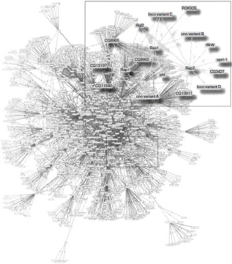
Initially biochemical methods like chemical cross-linking, combined fractionation during chromatography, and co-immunoprecipitation were used for investigation of protein–protein interactions. However, later such highly efficient and high-throughput experimental methods like yeast two-hybrid assay (Y2H), phage display, and tandem affinity purification-mass spectrometry (TAP-MS) were elaborated for interactome determination in various organisms [27-30]. Different microscopy techniques and different mathematical and computer methods also open broad possibilities for dynamic proteomics. These methods are described in detail in a number of reviews [27, 31, 32]. Therefore, here we shall describe only the main principles of these methods.
Yeast two-hybrid system. Yeast two-hybrid assay allows highly precise determination of protein–protein interactions in vivo. The method is based on the use of transcription factors characterized by modular structure and consisting of physically and functionally separable domains: DNA-binding domain (BD) and transcription activation domain (AD). Physical separation of BD and AD domains results in transcription factor inactivation. Activation of corresponding genes becomes possible upon reconstruction of transcription factor by fusion of these two domains with other two proteins X (called bait) or Y (called prey) that interact with each other [27]. DNA-binding domains of transcription factor GAL4 in S. cerevisiae or of lexA repressor in E. coli are usually used for creation of the two-hybrid system. The activation domain of GAL4 and protein B42 in S. cerevisiae and E. coli, respectively, are most often used as activation domains [33].
Yeast cells are transfected by two plasmids, the first of which contains nucleotide sequence encoding protein X linked to the BD domain, while the second encodes Y protein linked to the AD domain. As a result, DNA-binding domain together with X protein binds a certain sequence of reporter gene, whereas the AD domain together with Y protein binds another DNA region of this gene. Since DNA regions of a reporter gene, which bind regulatory proteins, are quite close to each other, no reporter gene activation is possible without physical interaction between X and Y proteins. The interaction between analyzed proteins can be inferred by the presence of the reporter gene expression products in yeast cells.
The yeast two-hybrid assay was first used by Fields and Song in 1989 during investigation in S. cerevisiae of GAL4 transcription factor that regulates expression of the gene encoding β-galactosidase that cleaves lactose to glucose and galactose [34]. Two functionally important domains are distinguished within GAL4—N-terminal DNA-binding domain, able to interact with operator sequence UASg, and C-terminal domain of transcription activation rich in acidic amino acids. The level of β-galactosidase expression is judged by intensity of coloring of enzyme-producing cell colonies after their incubation with a substrate. A high level of transcription activation is observed only if both hybrid proteins are present in the yeast cells. If X and Y proteins interact with each other, then functionally active protein GAL4 is reconstructed from two hybrid proteins and transcription activation takes place.
In the case of the LexA system, the accuracy of determination is provided by the use of yeast strains containing reporter genes carrying different numbers of LexA operator elements in the reporter gene promoters (usually lacZ and LEU2). More sensitive yeast strains have up to six LexA-binding elements, while less sensitive strains contain only two binding elements [27].
The yeast two-hybrid system was proposed as a method for screening libraries of proteins able to interact with some known protein used as a “bait”. The possibility of detection of physical interaction between different proteins allows using of this system for identification of specific amino acid residues responsible for interaction [35]. However, the Y2H method does not allow estimation of interaction with involvement of three and more proteins, except those in yeast. Moreover, this method not always makes it possible to estimate functional significance of observed physical protein–protein interactions.
Tandem affinity purification-mass spectrometry was introduced in 1999 by Rigaut et al. [29] as an original way for purification of proteins expressed under natural conditions at physiological concentrations. The method is based on the use of affinity tag attached to a target protein. Genes which encode tag components and a target protein is incorporated using retrovirus into a host cell capable of maintaining the target protein expression at a level close to physiological. The standard tag, used in yeast, consists of two immunoglobulin-G-binding fragments of Staphylococcus aureus protein A and sites sensitive to protease from tobacco mosaic virus and calmodulin-binding peptide. The target protein complex with the tag is isolated from the cell extract by a two-step procedure of affinity purification. The first step is based on binding of protein A to IgG-Sepharose, after which the complex undergoes action of the above-mentioned protease. The second step is based on partial binding of calmodulin-binding peptide, to calmodulin-Sepharose in the presence of calcium, and the complex is eluted by EDTA. The use of affinity tag allows rather rapid purification of protein complexes from a small number of cells without preliminary elucidation of protein composition of complexes and functions of individual proteins. In combination with mass spectrometry, this method provides for identification of proteins under study and their interactions [36].
Initially affinity purification was used in tandem with mass spectrometry for investigation of protein–protein interactions and functional organization of proteomes in simple organisms. For example, the work of a large group of German researchers resulted in expression of hundreds of proteins with affinity tag, and studying of their ability to form complexes with other proteins in S. cerevisiae [37]. This work led to purification of 589 protein complexes and prediction of functions for 344 various proteins.
Later the TAP-MS technique was applied to investigation of protein–protein interactions in different organisms including mammals [38]. Many varieties of affinity labels were proposed including those easily removable by specific peptidases [39, 40]. To enhance the efficiency of the method upon investigating protein–protein interactions in mammalian cells, a new tag based on G proteins that exhibit higher affinity to immunoglobulin G than protein A, were also developed. Streptavidin-binding peptide instead of calmodulin-binding peptide and biotin for elution can be used. This results in tenfold increase in the number of detectable protein complexes and higher specificity of the method. This approach makes it possible to use a small number of cells for purification of protein complexes that previously could not be purified by the standard TAP-MS technique [38].
Mass spectrometry is based on determination of molecular masses of peptides and proteins, by their preliminary ionization and distribution of obtained ions in an electric field depending on the mass-to-charge ratio (m/z) [30]. Two types of mild ionization are mostly used: matrix-assisted laser desorption/ionization (MALDI) and electrospray ionization (ESI). The MALDI method is the most popular in proteomic investigations. Here a sample containing peptides is mixed with molecules of specific matrix and then is subjected to an ionizing laser beam [41, 42].
In 1987 Karas and colleagues [43] were the first to demonstrate the possibility of matrix application for inhibition of fragmentation during analysis of nonvolatile organic compounds such as proteins and peptides. Matrix properties provide ionization of analyzed molecules and lowering destructive ability of laser irradiation. Emitted ions pass through the mass analyzer and moves to the detector that registers mass spectra of ions according to their mass-to-charge ratio (m/z). The spectra obtained are compared with spectral libraries using special computer programs. One of the MALDI varieties is MALDI-TOF (time of flight mass spectrometry) in which the time of ion flight through mass analyzer depends on mass and charge of substances under study [44, 45].
Another variety of mass spectrometry commonly used in proteomics studies is surface-enhanced laser-desorption/ionization (SELDI). In this method, the peptide-containing specimen is not mixed with the matrix but is applied on the surface of a special chip that is then placed in a vacuum cell where ionization of peptides or small proteins under study takes place [46, 47]. The resulting ions are accelerated towards the detector depending on their mass. A disadvantage of this method is impossibility of immediate identification of proteins represented in the mass spectra. Additional methods such as fractionation by ion-exchange chromatography and electrophoresis in polyacrylamide gel are used for protein identification [48].
The use of mass spectrometry, including its combination with other methods of analysis, is now a universal approach to identification of protein markers of various diseases, including tumors, cardiovascular, etc. [45, 46]. Mass spectrometry along with other methods of proteomic analysis such as two-dimensional electrophoresis, liquid chromatography, and protein biochips are also widely used for estimation of efficiency of different therapeutic approaches [49].
The phage display method is used for investigation of molecular interactions including protein–protein interactions and revealing of sites responsible for these interactions. It is based on the use of bacteriophages to correlate genes and encoded proteins. In this case, the recombinant viral DNA contains information about a protein molecule displayed in the phage capsid [50, 51]. Filamentous phages M13, fd, and f1 are used, because they are best suited for construction of recombinant DNA. The presence in the phage genome of a site insignificant for its vitality is most important for formation of hybrid DNA molecules. A foreign gene, encoding a certain protein or peptide (selective marker), that after synthesis is displayed on phage surface, is inserted into the phage genome. The recombinant DNA-carrying phage penetrates a bacterial cell (E. coli) where its amplification takes place. In this way, libraries are created that contain millions of phages, each of which contains in its capsid a unique protein (or peptide). Then the process called in vitro selection is carried out during which these libraries are screened by interaction of proteins exposed on the phage surface with a specific immobilized ligand.
The phage display method allows making correlation between phenotype and genotype, because the viral DNA contains information about the structure of the protein molecule expressed on the phage surface. Due to the simplicity and high rate of DNA sequence analysis, the phage display method allows rapid identification of proteins under study. Protein or peptide libraries can be also created using similar recombinant DNA technology.
One approach for estimation of protein–protein interactions is the use of phage clones that are able to specifically interact with polystyrene surface and carry genes encoding affinity labels, significantly increasing affinity to this surface [52]. Multienzyme complexes or the antigen–antibody complex are used as model systems. For example, cysteine synthase multienzyme complex in E. coli contains two enzymes, serine acetyl transferase (SAT) and O-acetylserine sulfohydrolase (OASS), which interact with each other when sulfur concentration is sufficient. In this case SAT activity increases, but OASS activity decreases, and this results in the formation of O-acetylserine. Immobilization on polystyrene surface of OASS hybrid enzyme, obtained either by genetic fusion or by chemical cross-linking with peptide label, increases the intensity of a signal estimated by immunoenzyme assay compared to that obtained upon immobilization of the enzyme alone. Moreover, when the peptide-labeled enzyme interacts first with SAT in solution with subsequent immobilization on polystyrene surface, the signal intensity increases even more owing to interaction of these enzymes without any steric hindrance.
Microscopy methods are presently widely used both for quantitative estimation of changes in concentrations and intracellular localization of different proteins and for qualitative investigation of protein–protein interactions. Protein complexes formed due to protein–protein interactions can be studied by detection within cells of the protein accumulation regions [53]. Modern methods of microscopy such as fluorescence microscopy and cryoelectron tomography can be used to visualize intracellular structures with resolution up to 4-5 nm [54, 55]. The average diameter of protein globule is 3-5 nm and that of macromolecular complexes is 10-100 nm. Therefore, combination of the two above-mentioned methods allows reconstruction of macromolecules, their complexes, and separate intracellular structures in native state [56, 57].
Combination of microscopy techniques with different experimental approaches and computational methods makes it possible not only to represent intracellular architecture as a whole, but to create a complete and comprehensive spatial molecular atlas of the intact cell [58]. For example, the human molecular atlas contains information about gene sets and profiles of protein expression in different normal and pathological tissues. In this atlas, proteins are classified by their functions as well as by tissues and biological fluids in which they are found [59].
Such methods of fluorescence microscopy as Forster’s inductive resonance transfer of electron excitation energy (FRET, fluorescence resonance energy transfer) and FLIM (fluorescence lifetime imaging microscopy) are also used to study protein–protein interactions. They make possible qualitative analysis of protein–protein interactions with investigation of dynamics of conformational changes occurring in proteins in space and time, and of amino acid residues involved in these interactions [60]. Fluorescence microscopy is based on measuring of different fluorescence characteristics like intensity, quenching time, polarization, and wavelength. The FRET method is based on measuring of energy amount emitted by the excited fluorophore molecule and transferred onto the acceptor molecule. Energy transfer is revealed by the increase in acceptor fluorescence accompanied by quenching of the fluorescence of the energy donor [61, 62]. In this case overlapping of the donor fluorescence spectrum with the acceptor absorption spectrum is a necessary condition for energy transfer. At the same time, this condition hinders spectral measurements, and this is a disadvantage of the method. Elimination of this disadvantage provides for the application of the FRET method for quantitative evaluation of the distance between interacting pairs of molecules both in vitro and in vivo, which is used in laser-scanning confocal microscopy. FLIM microscopy is based on the fluorescence lifetime measurements at each point of a spatial image [63]. It makes possible both estimation of interaction between proteins and analysis of local microenvironment of fluorophores, such as pH and concentration of different ions, oxygen, etc.
Microscopy methods that use fluorescent proteins as molecular markers are now actively developed. This allows observation in real time of dynamic alterations in localization and concentrations of thousands of proteins in different parts of a single isolated cell. To achieve this, a library of cell clones is created, each of which is fluorescently labeled on a certain protein. This approach on production of labeled proteins with retention of their natural localization and functions in a living cell was elaborated by Jarvik et al. in the second half of the 1990s and successfully tested in C. reinhardtii and D. melanogaster [64, 65]. Later the method was used to create libraries of cells labeled by fluorescent proteins in mammals, including humans [66].
A number of detailed experiments in real time investigation of dynamic alterations in localization and concentrations of different proteins during cell proliferation were carried out by the group of Alon et al. [67, 68]. Human lung carcinoma H1299 cells were infected by retrovirus carrying the gene encoding yellow fluorescent protein (YFP). A library of over 1200 cell clones was created, each of which could express its fluorescently labeled protein. Cells containing the certain labeled protein were selected using flow cytometry, and then the labeled proteins were identified. Real-time fluorescent microscopy made it possible to observe dynamics of changes in localization and concentrations of 20 nuclear proteins during the cell cycle. It was found that different proteins are characterized by different dynamics of accumulation in the cell nucleus. Dynamics of topoisomerase TOP1 accumulation had sinusoidal character with maximum accumulation in the nucleus in S phase of the cell cycle, whereas other proteins were characterized by maximum accumulation in the nucleus in G1 or G2 phases. This method revealed the existence of distinctions in localization of different proteins during the cell cycle.
The use of such technologies also allows studying drug effects on protein dynamics in tumor cells, the mechanism of drug resistance in cells, and the role of different proteins in cell survival. For example, studying dynamics of about 1200 different proteins of human lung carcinoma H1299 cells under exposure to antitumor drug camptothecin, which blocks topoisomerase-1 in complexes with DNA accompanied by DNA breaks and gene transcription inhibition, made it possible to reveal changes in different protein concentrations and localization in response to this drug [68]. The cells intensively divided during 24 h with cell cycle duration of about 20 h. However, within 10 h after drug addition, lowering of cell motility and inhibition of their division were observed along with morphological changes indicative of cell death. In 36 h, the described changes involved 15% of all cells.
In this case, almost 76% of changes in protein fluorescence intensity were observed in the course of time. Groups of functionally related proteins showed similar dynamics of changes in their intracellular localization and concentrations. It was shown that ribosomal proteins underwent rapid degradation, whereas cytoskeleton proteins and enzymes were destroyed rather slowly. In this case, helicases and apoptosis regulating proteins such as Bcl2-associated proteins BAG2 and BAG3, as well as PDCD5 demonstrated the slowest degradation in response to this drug [68]. Topoisomerase-1 underwent the most rapid degradation, and the localization of the enzyme was changed significantly. Concentrations of two proteins (RNA helicase and DDX5 protein) increased significantly in the cells exhibiting tendency to survival, while it decreased in the cells that underwent morphological changes resulting in their death.
Thus, it was shown that distinctions in cell reactions to drugs are defined by differences in changes in concentration and localization of various proteins. The great advantage of such microscopy techniques is the possibility to study processes happening under living cell conditions with preservation of natural functions of intracellular macromolecules. Besides, they can be used to observe processes taking place in real time in a single isolated cell.
Computer-based methods. The use of a combination of different experimental and theoretical methods is a possible way of overcoming difficulties emerging during studies of protein–protein interactions [69-73]. In this case, it is necessary to separate real results from false-positive ones, which requires elaboration of systems for estimation of data reliability. Because of labor-consumption and expense of high-throughput experimental methods, the most important role belongs to various computer methods of prediction of protein–protein interactions [74]. For this purpose, information on the structure of genes and proteins encoded by them is used along with available data about protein functions and possible functional relationships between them.
In recent years, different computer methods of data clustering have been elaborated that makes it possible to estimate the extent of functional similarity between proteins and to reveal protein complexes. Clusters obtained represent spatial and functional protein associations. They are compared with protein complexes experimentally confirmed and described in special annotated databases [75]. Some of these approaches can also reveal functionally important modules in interactome maps.
Computer investigation of protein complexes requires highly efficient computational methods and development of new algorithms such as MCL (Markov Clustering), RNSC (Restricted Neighborhood Search Clustering), SPC (Super Paramagnetic Clustering), and MCODE (Molecular Complex Detection) [76, 77]. Recently significant progress has been achieved in the broad-scale mapping of interactomes of various organisms as well as in creation of databases and special tools for analysis of information stored in them.
Modern databases contain information about many hundred thousand interactions formed by several thousand proteins in tens of biological species [78-80]. For example, database BioGRID (Biological General Repository for Interaction Datasets) contains to date information on approximately 198 thousand interactions for six biological species [81]. Such databases contain information about interacting pairs of proteins either obtained by experimental methods or determined by homology-based prediction using computer methods. The purpose of such databases as DIP (Database of Interacting Proteins), BIND (Biomolecular Interaction Network Database), and INTERACT is integration of a great amount of experimental data, providing easy access to them, and the possibility of their visualization. Databases are also furnished with tools for estimation of reliability of experimental results. They are widely used for construction and analysis of protein interaction networks that form a basis for functioning of living cells.
Presently created databases not only contain information about interacting partners, but also make possible detailed structural analysis of regions responsible for interaction [82-84]. For example, SCOWLP (Structural Characterization Of Water, Ligands, and Proteins) database contains information about amino acid residues and groups of atoms involved in interactions. Owing to this, it provides for detailed analysis of interactions between proteins, domains, and peptide motifs of different proteins as well as of their interactions with solvent [82, 83]. Another example is the global interactome map PSIMAP (Protein Structural Interactome Map), which is constructed using data on domain–domain interactions with involvement of all proteins for which three-dimensional (3D) structures are experimentally established and presented in PDB (Protein Data Bank). The PSIMAP algorithm makes possible calculation of Euclidean distances between amino acid residues of two interacting domains within different proteins [85]. Two domains are considered as interacting if at least five amino acid residues are at a distance less than 5 Å (the 5-5 rule). This algorithm can be used to predict interacting partners by homology of amino acid sequences of proteins and their structural domains. Information on interacting partners is contained in the PSIbase database.
Mapping Interactomes of Different Biological Species
The most complete map compiled for prokaryotic organisms is that of protein–protein interactions of pathogenic microorganism Campylobacter jejuni [86]. The use of Y2H method has revealed and reproduced about 12,000 interacting pairs, including proteins involved in regulation of different biological events like chemotaxis. Another intensively studied prokaryote is E. coli, which is considered as a model microorganism for investigation of prokaryotic interactomes [87]. However, data obtained for this organism by different groups of authors are contradictory. According to different authors, the size of the E. coli interactome varies from several thousands to several tens of thousands of interactions.
The use of approaches of functional and comparative genomics enabled prediction of the existence of over 78,000 paired interactions in E. coli [88]. Moreover, it was shown that proteins involved in replication, transcription, translation, DNA repair, and cell wall synthesis are characterized by a high density of interconnections with each other. The interactome of E. coli cell wall is studied especially intensively [89]. The database Bacteriome.org containing information about interactomes of this organism was created on the basis of data obtained using experimental proteomic techniques and methods of comparative and functional genomics [90]. It assures an integrated view of the E. coli interactome and allows users to reveal and analyze structural, functional, and evolutionary relationships between groups of interacting proteins. This database now contains information about over 5000 experimentally confirmed interactions with involvement of over a thousand proteins.
A classic subject in proteomic investigations is the yeast S. cerevisiae, for which the most complete interactome data for unicellular eukaryotic organism were obtained. However, results of different groups of authors obtained for S. cerevisiae using different experimental methods are contradictory [91, 92]. The most precise data on each protein copy number and intracellular localization were obtained by combination of different methods [93, 94]. A total of 7123 interactions with involvement of 2708 proteins were detected using the TAP-MS technique [95]. Data clustering using the Markov algorithm revealed 547 protein complexes, each of which contained on average 4.9 proteins.
To obtain more precise and reliable data, a large group of authors elaborated a new “empirically controlled” mapping system [94]. This system made it possible to choose from literature data a pool of paired interactions, which were then tested using the Y2H and TAP-MS methods. This allowed creation of the “second generation” of low-productive but high-quality data. This approach produced high-quality results covering about 20% of the interactome of S. cerevisiae.
Mapping protein–protein interactions in D. melanogaster is considered as a model system for investigation of biology, development, and mechanisms of emergence of human diseases. The Y2H system was used for screening D. melanogaster cDNA libraries to reveal interacting partners for 102 proteins used as “bait” [96]. Most of these proteins were orthologs of human tumor-associated or signaling proteins. About 2300 paired interactions were revealed, and 710 of them were estimated as of high confidence. Estimation of reliability of the results and revealing the interacting domains have contributed to improvement of data concerning already known protein complexes and prediction of new ones. Interacting pair mapping for the cell cycle protein regulators in D. melanogaster revealed 1814 interactions for 488 proteins [97]. Special annotated databases containing information about experimentally obtained and computer-predicted data on physical protein–protein interactions were also created for the given biological species [98-100].
Human interactome mapping is now just at the initial stage of investigation. Statistical estimation of the human interactome size suggests that it may reach 650,000 interactions [20]. However, according to Venkatesan et al. [101] the human interactome is represented by 130,000 interactions, and the interacting partners are still not found for the overwhelming majority of proteins [101]. These data were obtained using the new above-described “empirically controlled” approach. This approach was used to estimate qualitative parameters of methods used for studying protein–protein interactions. These parameters included sensitivity, completeness of screening, the number of revealed interactions, and the accuracy of the method (number of artifacts). Works of this group of authors showed that two-hybrid analysis (Y2H) is most suitable for estimation of protein–protein interactions in humans. The constructed interactome maps appeared to be more precise compared to those obtained by analysis of published data. This is due to the fact that in the latter case only results of a single publication were used.
To date the use of Y2H assay and affinity purification combined with bioinformatics approaches has revealed interacting partners for proteins of some tissues including brain, kidneys, erythrocytes, etc. [102-104]. Accumulated experimental data are included in special databases like HPID (Human Protein Interaction Database) and OPHID (Online Predicted Human Interaction Database), which contain information about protein–protein interactions characteristic of humans. These databases are created using both experimental results and those predicted by homology with interacting pairs revealed in simpler model organisms [105, 106].
Studying of protein–protein interactions and revealing interacting partners specific for a certain pathology is an important tool for elucidation of mechanisms of emergence and development of a disease. Disturbance in synthesis of components of the signal transduction pathways or mutation in genes encoding synthesis of these proteins is often the factor responsible for emergence of diseases including tumors [107]. The use of affinity purification combined with mass spectrometry revealed 221 molecular complexes formed by tumor necrosis factor α (TNF-α), its receptor, and intracellular effectors [108]. TNF-α initiates a cascade mechanism of signal transduction that results in activation of nuclear factor (NF-κB) playing the role of transcription factor and regulating expression of a number of genes responsible for cell proliferation and survival [109]. Distortion of this function is the basis for development of many pathological processes within an organism such as tumor growth, inflammatory and autoimmune diseases, etc. For example, nuclear factor NF-κB induces expression of genes that encode antiapoptotic proteins TRAF1 and TRAF2, thus regulating activity of the caspase family enzymes. Mutations in the gene encoding NF-κB or in genes regulating its activity are observed in a number of tumors [110].
Works have begun on revealing interacting protein pairs associated with neurodegenerative diseases, sickle cell anemia, schizophrenia, etc. [111-113]. Interactome mapping in neurodegenerative diseases like Alzheimer, Parkinson, and Huntington diseases, amyotrophic lateral sclerosis, as well as prion diseases revealed that proteins associated with them are characterized by the presence of common interacting partners [112]. Nineteen proteins common for all these pathologies were revealed, and most of them appeared to be apoptosis regulators or participants of signal transduction mediated by the mitogen-activated protein kinase (MAPK). In addition, domains characteristic of all these proteins like SH2 (Src homology 2) and phosphotyrosine-binding (PTB) domain were revealed within these proteins.
PROTEIN INTERACTION NETWORKS
A group of physically interacting proteins forms a protein network. Protein interaction networks are a variety of molecular networks, among which there are also gene networks that include genes, regulatory RNAs, and transcription factors; metabolic networks consisting of substrates and products of biochemical reactions; and networks of signaling molecules including receptors, their ligands, and intracellular effectors [114-118]. Classification of molecular networks mentioned above is conditional because transcription factors and enzymes catalyzing biochemical reactions are proteins by their nature. Also, there is a functional connection between components of different types of molecular networks. Thus, on one side, expression of any gene is controlled by external signals mediated by protein receptors and their intracellular effectors. Both proteins and low-molecular-weight intermediates of metabolic pathways can serve as ligands for the receptors. Some intracellular effectors, components of signaling networks, can penetrate into the cell nucleus and play the role of transcription factors that control gene expression. On the other side, the rate of biochemical reactions depends on activity of enzymes—gene products. Enzyme activity, in turn, can be regulated by low-molecular-weight substrates or products of biochemical reactions.
Among all the above-mentioned types of molecular networks, signaling networks are the most complicated ones with regard to functional interrelationships between components. The components of signaling network are able to interact with each other both physically (as in the case of ligand–receptor interaction) and by involvement in chemical modifications of other components (for example, protein kinases), or in gene expression regulation (intracellular effectors). Thus, proteins can be involved in different types of molecular networks as their structure–functional components. However, a special type of molecular networks, namely, protein networks, is used for modeling physical protein–protein interactions.
Organization Principles and Properties of Protein Networks
Molecular networks, along with networks of nerve filaments, blood and lymph vessels, etc., belong to biological networks. Both biological and non-biological networks (such as social and technological ones) are types of complex networks, the description of which requires methods of mathematical analysis and graph theory [119, 120]. As shown by recent studies, all types of complex networks, both biological and non-biological, are based on the same structural principle. Using the graph method, complex networks can be represented as a combination of nodes linked to each other by directed and non-directed edges. The network components are located in the nodes, and edges indicate the links between them. Regulatory gene and metabolic networks can be represented in the form of graphs with directed edges in which the link direction points either to the gene under regulatory effect of a transcription factor or direction of a reaction [119, 120]. Networks of signaling molecules may be represented as graphs both with directed and non-directed edges. Since both partners are equally involved in protein–protein interactions, protein networks are shown in the form of graphs in which adjacent nodes are bound to each other by non-directed edges (Fig. 2).
Global structure of complex networks can be represented by large graphs consisting of thousands of interlinked nodes. In description of local structure, separate parts of networks (subnetworks) that can be represented only by several nodes and links between them are considered [121]. Among global parameters used for description of complex network organization principles, topological and dynamic characteristics are distinguished. Knowledge of protein network architecture and dynamics obtained using these parameters makes it possible to reveal the main principles of functioning of the intracellular structure [122]. Topological characteristics include the number of nodes within the network and the number of edges at each node (i.e. the number of adjacent nodes linked to it), an average path length or network diameter, its density and heterogeneity, and clustering coefficient. Among dynamic parameters are the network resistance to any external effects and the frequency and amplitude of oscillations emerging in the network.Fig. 2. Types of complex networks (according to [131]). a) Schematic representation (on the left) and configuration (on the right) of scale-free network. Gray circles (on the left) correspond to hubs. b) Schematic representation (on the left) and configuration (on the right) of a modular network. Here all nodes have an equal number of links with adjacent nodes. Such a network is free of hubs. c) Schematic representation (on the left) and configuration (on the right) of hierarchically and modularly organized scale-free network. The figure is the courtesy of A.-L. Barabasi [131].
An important parameter of complex networks is the path length or the distance between two nodes within the network, characterized by some number of other nodes between them. The shortest distance between two nodes is the shortest path length. The average path length within the network or its diameter is determined by calculation of average lengths of all such paths between all node pairs. It has been shown that protein networks exhibit properties of the “small world” with diameter (i.e. an average path length) equal to 4-5 nodes. Networks with the “small world” properties were first described by Watts and Strogatz [123] who found that distances between nodes in many biological and non-biological networks are not long. As a result, processes taking place in most complex networks are characterized by rapid dynamics and by the effect of signal enhancement and synchronization. Networks with “small world” properties are in intermediate position between regular graphs, which have tendency to minimization of number of links, and graphs with random architecture, which are characterized by numerous links [124]. Such networks show the presence of hubs (hub is center or focus), i.e. of a small number of nodes with numerous links.
Clustering coefficient is the measure of the ability of a node to form regions with high link density, i.e. clusters [124]. The mean value of clustering coefficient for all nodes corresponds to clustering coefficient of the whole network. In real networks for the node with degree k, clustering coefficient C(k) is proportional to k–1 where k shows the number of adjacent linked nodes (k = 1, 2, 3…). Clustering coefficient is the measure of the network organization heterogeneity and hierarchy. The network hierarchy means the existence of a multilevel form of organization with strict subordination of lower levels to the higher ones. Each of the groups (clusters), characterized by a high density of internode links, is a structure–functional module within the network.
Usually two main types of models, namely random geometry and scale-free graphs, are used to characterize the heterogeneity of complex networks [125]. Data of different groups of authors that characterize architecture of protein networks are ambiguous and contradictory. Przulj et al. [126] used different models for global and local analysis of protein networks in S. cerevisiae and D. melanogaster and showed that random geometry graphs are better suited for description of physical protein–protein interactions. The random geometry networks are described by the G(n,r) graph consisting of n number of nodes represented by n independent dots, equally and randomly distributed in metric space, at distance r between them. Such networks are rather homogeneous, and quantitative estimation of any node link probabilities is characterized by a binomial distribution [127]. In the case of large networks, density of probability that a certain node has k links is characterized by a Poisson distribution (Fig. 3):
![]()
In this case, each node has approximately equal probability to be linked to any other node.
However, systemic analysis of the S. cerevisiae, C. elegans, and D. melanogaster protein network topological characteristics, carried out by different research groups, revealed the scale-free character of most networks and the high extent of their clustering [128, 129]. In this case, the scale-free character of protein interaction networks means existence of degree distribution [128]. The degree distribution function for scale-free networks can be assigned as P(k) = Ak–γ, where P(k) is the density of linkage probability between adjacent nodes, A is a constant, γ index is usually 2 < γ < 3 (most often it is 2.2) for all organisms [122]. Such distribution function is indicative of network heterogeneity, i.e. practically of impossibility of finding in it a typical node suitable for characterization of all the other nodes in the network.Fig. 3. Comparative graphs of degree distribution functions for protein networks with random geometry (squares) and “scale-free” protein networks (circles). Linear graphs are given on the left, graphs in logarithmic scale are on the right (according to [85]). The bell-shaped graph of distribution function for protein networks with random geometry points to static homogeneity of such networks. The graph of distribution function for the “scale-free” protein networks follows formula P(k) = Ak–3 and characterizes the network heterogeneity. The character of the decrease in the distribution function suggests existence of numerous nodes with a small number of links and small number of hubs with numerous links.
The key property of the scale-free architecture is the presence of hubs, i.e. nodes with high density of linkages, whereas most nodes are characterized by a small number of links (Fig. 2). However, a small number of hubs provides for stability of the whole cell by uniting all the nodes in the network. Experiments on hub removal from protein and metabolic networks in D. melanogaster are indicative of the role of hubs [129]. Networks with scale-free architecture appeared to be resistant to random removal of nodes. Even after removal of a large number of randomly chosen nodes, links between the remaining ones in the network are not disturbed and the network topology does not change. However, the removal of hubs alone results in 2-3-fold increase of the network diameter.
Biological significance of hub removal was shown in experiments on S. cerevisiae which demonstrated that knockout of genes encoding proteins located in hubs was accompanied by increased lethality. However, removal of genes encoding proteins located in other nodes had no such effect [130]. Such network property was called the lethality–centrality. These data show that proteins located in hubs are necessary for the organism survival and as a whole they can be functionally more important than proteins located in other nodes.
The hierarchy serves as the fundamental characteristics of many complex networks and shows that large groups of nodes in such networks consist of smaller groups (modules) organized in hierarchical order [131]. Modules can be defined as structurally independent units consisting of several components and capable of relatively independent functioning. In this case, links between nodes belonging to different modules are characterized by lower density than links between nodes of the same module.
The hypothesis on modular organization of protein networks was proposed on the basis of systems analysis using bioinformatics resources of data on expression, intracellular localization, evolution, structure, and functions of proteins and their interacting partners [132-135]. Although some authors follow the opinion on absence of biological significance of the protein network modules [135], quite a number of data are in favor of their functionality. Comparison of experimental methods and functional annotation of genes has shown the possibility of existence of two types of modules in protein networks: (i) protein complexes and (ii) dynamic functional modules that combine proteins involved, for example, in cell cycle regulation [136].
The existence of strong correlation between structure, function, and intracellular localization of proteins that are involved in network formation has been demonstrated in a number of works [137, 138]. For example, information about interacting pairs of proteins obtained from the DIP database was used to construct protein networks for S. cerevisiae. It was shown using the Girvan–Newman (G-N) algorithm and MoNet program that these networks are organized in 86 simple modules, each of which consists of more than three proteins [133]. Each module was represented mainly by functionally interrelated proteins. Other authors used an integrated approach with involvement of data obtained by gene expression analysis using oligonucleotide chips, along with proteomics results, and revealed 266 functional modules in yeast protein networks [139]. The probability of interaction between proteins of functionally different modules was low [140].
It was shown using computer modeling that modular organization of molecular networks can be a result of gene duplication. Revealing the fact that evolution of protein networks takes place at the level of modules leads to necessity of calculation of degree of conservation between two interacting protein pairs. This is achieved by comparison of primary structures of network proteins by alignment as well as by comparison of different network architecture [141, 142]. In this connection, special algorithms for searching for similar networks among a set of molecular networks in different biological species or within one species have been proposed in some works.
Construction of spatial (3D) models and their visualization are used to characterize topology of protein networks [143, 144]. Such models are created using such proteomics data as intracellular localization of proteins, approximate number of copies of each protein within a cell, their physicochemical characteristics, and data on protein posttranslational modifications and orthologs. Special databases contain information about organelle-specific protein–protein interactions, which is also used for three-dimensional modeling [145-147].
Unlike static graphs, really existing networks are characterized by dynamic properties, i.e. by changes in space and time. Temporal parameters of protein–protein interactions can be studied by gene expression analysis using oligonucleotide chips. Calculation of correlation between expression of proteins located in hubs and that of their interacting partners made it possible to distinguish two types of proteins located in hubs [148]. The high extent of co-expression of the proteins was specific for the first type, while low extent was specific for the second. Hubs of the first type are static (party hubs), and the second type hubs are dynamic (date hubs). It was supposed that proteins located in static hubs are characterized by a constant set of interacting partners, while proteins in dynamic hubs interact with different partners at different times. Probably the first type hubs plays a local role in networks and are characterized by strong links within a functional module. The second ones are of global significance because they bind different functional modules with each other. It was shown that the removal of dynamic hubs results in more severe consequences (increasing of diameter and disintegration of a network) compared to the removal of static hubs. However, soon it became clear that increased lethality was caused by removal of either type of hubs [149, 150].
Among important dynamic characteristics of complex networks, their robustness to any factor and periodic oscillations should be distinguished. These oscillations are indicative of cyclic character of intracellular processes. Cycles of cell activity are controlled by cascade mechanisms following the principle of direct and feedback regulation [151, 152]. The activity of a cell depends on coordinated functioning of genes and their protein products as well as low-molecular-weight metabolites involved in regulatory pathways. Dynamic characteristics of protein networks and methods of their modeling will be considered in the section “Methods of Dynamic Modeling in silico”.
Biomedical Significance of Protein Interaction Network Analysis
Analysis of protein interaction networks can be used to solve a number of problems in fundamental medicine, among which there are revealing and understanding of mechanisms of arising and development of tumor, neurodegenerative, cardiovascular, and autoimmune diseases, as well as search for molecular targets for drugs.
In a number of works using the OPHID database containing experimentally confirmed or predicted information on protein–protein interactions, graphs illustrating protein networks with involvement of products of genes expressed in tumors were constructed. It was shown that networks of tumor-associated protein products of genes characterized by different regulatory pathways, are larger than the those formed by a random set of proteins [153]. This suggests existence of functional interrelations between proteins. A carcinogenesis model based on analysis of protein interaction networks was proposed that considers it as a process specifically organized at the molecular level and characterized by decreased expression of topologically and functionally associated proteins synchronized with increased expression of other proteins [154].
Presently available data on the disease-associated protein networks are incomplete and ambiguous. It has been also shown that proteins associated with similar diseases are characterized by higher probability of physical interaction with each other. A hypothesis concerning existence in protein networks of functional modules specific for different diseases was put forward. According to this hypothesis, proteins necessary for embryonic development and normal cell functioning are synthesized in different organs and are located in hubs of protein networks, while the majority of disease-associated proteins are located in the network periphery [155].
However, it has been shown in a number of works that tumor-associated proteins are characterized by a high density of links and in contrast to normal proteins, they are located in central hubs and contain numerous structural domains involved in protein–protein interactions [156-158]. Tumor-associated proteins contain double the number of interacting partners compared to normal proteins. The presence of numerous interacting partners can be responsible for the central role of these proteins in the network and means their higher involvement in intracellular pathophysiological processes. Wachi et al. mapped in the human interactome protein products of 360 genes with increased expression and of 270 genes with lowered expression in lung cancer [159]. It was found that over-expressed proteins are characterized by a larger number of links compared to proteins demonstrating decreased expression. Thus, a high extent of centralization was shown for proteins with increased synthesis in tumor compared to normal tissue.
Analysis of the protein network modules shows that they contain products of co-regulated and functionally interrelated genes and can be associated, for example, with gene polymorphism or with mechanisms of emergence of a disease [160]. Moreover, proteins exhibiting their activity only within a certain functional module can be considered as markers of this module or as potential drug targets. Revealing of tumor-associated genes and their protein products interacting with known proteins, which represent tumor biomarkers, can contribute to elaboration of a new strategy in diagnosis of diseases [161].
Application of special computer programs such as Cytoscape can be used to comparatively visualize experimental data and to use them together with information contained in annotated databases on molecular networks [162]. For example, it was shown using this approach that proteins involved in regulation of epithelial–mesenchymal transition initiated in kidney cells by TGF-β1 form a common network [163]. Analysis of gene ontology revealed in signaling pathways hyperexpression of proteins that control morphogenesis and embryonic development.
Analysis of molecular networks also contributes to understanding of mechanisms underlying emergence of complex diseases caused by genetic and non-genetic factors, e.g. environmental factors, nutrition, etc. [164]. On this basis, a new approach to disease diagnosis and classification is proposed. Analysis of molecular networks also allows revealing new potential drug targets and detection of drug resistance of cells. This actually provides for new approaches to the treatment of diseases. For example, comparison of networks formed by proteins involved in apoptosis of HeLa cells and normal human fibroblasts contributed both to elucidation of the mechanism of apoptosis and to the search for potential drug targets [165]. The existence of numerous interactions (841) in tumor (HeLa) and normal cells was detected. About 18.7% of these interactions were present in tumor cells and absent in normal cells. On the contrary, approximately the same number of interactions were revealed in normal cells and were not found in tumor ones. As a whole, these interactions were determined as potential drug targets. It was supposed that Bcl2, PT53 proteins, and caspase-3 can be drug targets. An interesting result of this work is also revealing of proteins located in static and dynamic hubs of protein networks. Caspase-3 was shown to be located in dynamic hubs of networks formed by proteins responsible for apoptosis of normal and tumor cells. Caspase-2 and caspase-9 were responsible for topological distinctions between the networks. More detailed analysis of the role of molecular networks in elucidation of disease mechanisms, diagnosis, and classification is described in several reviews [155, 156, 166].
Protein Complexes
Protein–protein interactions form the basis of functionally important stable protein complexes. Microscopy methods revealed that protein molecules are irregularly distributed in cytoplasm of living cell and exist there as aggregates [167-169]. The content of macromolecules in such aggregates can vary from 50 to 400 g/liter, so protein–ligand and protein–protein interactions, conformational transitions of the macromolecules, as well as formation of self-organized supramolecular structures become easier [170].
modern proteomics methods provide quite detailed characterization of composition and organization of these intracellular structures. The protein complexes are key supramolecular structures in which products of several genes are integrated and which are mainly intended to carry out some interrelated functions. They may be a multienzyme complex that catalyzes a chain of biochemical reactions or a complex of proteins that are participants of a signal transduction pathway.
Protein complexes are formed due to the fact that each protein molecule can simultaneously have several protein-binding sites. For example, studying linker protein for T lymphocyte activation (LAT) has shown that four sites containing phosphorylated tyrosine residues interact with SH2 domains of signaling pathway adapter proteins [171]. This stimulates formation of protein complexes, making easier signal transduction from the membrane into cells, which is the basis for normal maturation and differentiation of immunocompetent cells. Mutations that lead to replacement of tyrosine residues involved in binding of different adapter proteins cause disturbances in T lymphocyte differentiation and B lymphocyte maturation.
In a protein complex a core formed by a constant set of proteins is surrounded by peripheral part of variable proteins. The cooperativity in interaction between different proteins within such complex was shown, and this is determined by different affinity and specificity of their binding to each other [172]. The character and mechanism of association and dissociation of such complexes mainly depends on their size. Investigations in S. cerevisiae showed exponential decrease in distribution in size of protein complexes. However, studying dynamics of protein complexes has shown that their association can be independent of the complex size [173].
Some proteins are able to be simultaneously involved in formation of several complexes, which can be explained by multifunctionality and multimodularity of these proteins. Since protein complexes are mainly intended for carrying out a certain function, then multifunctional proteins can realize different functions within various complexes with involvement of different functional modules.
STRUCTURAL AND FUNCTIONAL MODULES RESPONSIBLE FOR PROTEIN
INTERACTIONS
Revealing of the same proteins within different protein complexes can be explained by the presence of several functionally important sites including those responsible for protein–protein interactions. This means multimodularity of protein structure. Recent studies show that modularity is a universal property of living beings and is revealed at all levels of their organization. As mentioned above, modularity is characteristic of also protein networks, and this determines complexity and hierarchic character of their organization.
Modular organization can be also characteristic of individual proteins, and this means that a protein molecule can consist of several (and even of a great number) of structurally and functionally independent elements (domains and motifs). In this case, each module is responsible for a protein function and can function independently of others. As a result, a protein molecule acquires the ability to carry out a whole complex of different functions; such proteins are called multimodular and polyfunctional [17, 18]. Probably these functions are interrelated, i.e. the set of functional modules of any particular protein is evidently formed nonrandomly. The cell type, its microenvironment, physiological and pathophysiological cell condition, as well as microenvironment of the protein molecule itself define which protein module can be involved in protein functioning. Mosaic structure, multimodularity, and multifunctionality are probably characteristic of most eukaryotic proteins.
Structurally similar modules can appear within different proteins, probably causing similarity of some of their functions. Molecules of different proteins can be constructed by combination of a limited set of structurally and functionally independent modules, which in turn is determined by physiological (biological) role of a protein [174]. This hypothesis is confirmed by experiments on creation of artificial multifunctional proteins formed by different combinations of peptide motifs with already known function. These experiments showed (i) compact packing of a protein molecule is not a necessary condition for its function realization; (ii) function of a motif depends on composition and arrangement of a set of motifs [175]. Moreover, it appeared that rearrangements of different motifs can produce proteins with absolutely different functions.
Protein multimodularity can result in significant complication of the character of a protein interaction network [176]. If multimodular, multifunctional proteins are located in the nodes of protein networks, each node can be represented not by a separate protein but by its functional module, and internodal links become interlaced. In this connection, it seems important to design structure–functional maps for multimodular and multifunctional proteins in order to reveal sites responsible for any function, including protein–protein interactions.
It has been shown experimentally that protein–protein interactions involve domains of some proteins and corresponding short linear peptide motifs of other proteins. If a protein contains several domains for interaction or several binding motifs, it can simultaneously interact with several proteins, and this results in formation of protein complexes. Examples of domains participating in protein–protein interactions are SH2 and PTB domains that bind to phosphorylated tyrosine residues within receptors, or SH3 and WW domains that react with proline-rich protein motifs [177-179].
One model system for studying protein–protein interactions is the SH3 domain interaction with proteins that contain proline-rich domains [180, 181]. Protein networks resulting from interaction of different proteins with SH3 domains were revealed in S. cerevisiae, in which 28 proteins containing such domains were detected. The use of the Y2H technique revealed 233 interactions with involvement of 145 proteins, and the phage display technique revealed 394 interactions between 206 proteins.
Structural analysis of the SH3 domain has shown that its polypeptide chain contains about 50-70 amino acid residues and is organized in five β-folded structures. To date over 1500 different SH3 domains are known and PXXP motif is their classical binding site (where P is proline and X is any amino acid) [182-184]. SH3 domains are present within such enzymes as kinases, lipase, or GTPase. The best studied are functions of SH3 domains in adapter proteins like c-Src or Grb2, participating in the signal transduction from membrane receptors to their cytoplasmic effectors. For example, proline-enriched tyrosine phosphatase (PEP) binds to SH3 domain of cytoplasmic tyrosine kinase Csk (C-terminal Src kinase) with involvement of a PXXP motif [184]. It was shown that the amino acid residues including A40, T42, and L43 within the SH3 domain and forming hydrophobic bonds with PEP take part in this interaction. Another example is interaction of PXXP motifs of dynamin-1 and dynamin-2 proteins with purified SH3 domains of such proteins as c-Src, Grb2, and intersectin. Studying of kinetics of such interactions has shown that different SH3 domains can bind to the same proline-rich domain. Evidently, under conditions in vivo, several SH3 domains can compete for binding with PXXP motifs [185].
Short linear motifs are sequences mainly consisting of 3-10 amino acid residues responsible for a protein function [186]. They are involved in protein–protein interactions, interactions of the protein–ligand and protein–nucleic acid type, and can serve as sites of posttranslational protein modifications such as phosphorylation, glycosylation, etc. The first linear motifs found within proteins were KDEL and HDEL sequences that are functional sites of proteins of endoplasmic reticulum and are responsible for prevention of secretion of these proteins [187]. It has been also shown that the KKXX motif found in cytoplasmic domain of transmembrane proteins functions as a signal site responsible for return of proteins from Golgi apparatus into cisternae of endoplasmic reticulum [188, 189].
It is difficult to reveal short linear motifs consisting of a small number of amino acid residues by comparison of the protein primary sequences. So, such labor-consuming and multistep experimental methods as point mutagenesis or phage display are usually used for revealing short linear motifs and the role of any amino acid residues in their functioning. There are now appearing new bioinformatics resources for detection of short linear motifs within proteins [190, 191]. Computer methods for binding motif revealing are based on the use of databases on protein–protein interactions and extraction of motifs common for the group of proteins interacting with each other. Special algorithms like D-MOTIF, D-STAR, MEME, Gibbs Sampler, PRATT, and TEIRESIAS can be used for this purpose [192-195]. This approach is based on the assumption that proteins having common interacting partners should be characterized by existence of similar motifs. Presently appearing databases contain information about all known functionally important protein sites. For example, the SCOWLP database contains information about over 9000 protein-binding sites of proteins belonging to over 2500 families. It appeared that members of 65% of families contain more than one binding site and 22% of sites are involved in formation of complexes with several proteins belonging to different families [82, 83].
Methods of comparative genomics and gene clustering were used for detection of functionally important oligopeptides in proteins of seven biological species [196]. This approach revealed tri- and tetrapeptides such as signaling motifs SKL, KDEL/HDEL, and KKXX and allowed predicting new motifs that may be of functional significance. Special tools allow simultaneous determination of potential contacts between amino acid residues of different polypeptide chains [197]. For example, the Con-Struct Map algorithm allows investigation of changes in protein spatial structure resulted from amino acid replacements or, on the contrary, determination of conserved residues important for interaction. This algorithm also provides a possibility to study structure–function relationships between unrelated and non-homologous proteins.
METHODS OF DYNAMIC MODELING in silico
Mathematical and Computer Modeling
Static graphs used for description of topology and properties of protein networks do not reflect conformational and dynamic characteristics of macromolecular complexes and multiplicity of protein functions. Because of this, it is now important to develop methods for description of conformational and dynamic properties of protein complexes and to create dynamic models of intracellular processes. The following methods are used in systems biology: (i) mathematical modeling using a system of equations, or (ii) computer modeling based on special algorithms for construction, design, and visualization of intra- and intercellular processes and events [198-200].
Mathematical modeling has become an important tool for an integrated approach to understand complicated intra- and intercellular processes [201]. It becomes widely used for description of events and processes taking place in a living cell and serves as a universal language for interpreting experimental data and prediction of properties and behavior of biomacromolecules under various conditions. Biomolecular systems including ligands, receptors, adapter proteins, and intracellular effectors of signaling pathways are best studied from the point of view of mathematical modeling [202]. For example, an attempt using this approach was undertaken to elucidate mechanisms of fibroblast proliferation in response to epidermal growth factor (EGF) [203]. Using kinetic parameters of the growth factor binding to its receptor as well as dynamic parameters of the ligand–receptor complex internalization, degradation, and recycling, and DNA synthesis, it became possible to explain many available experimental data and to predict new properties of this signal system. A similar situation exists in investigation of dynamic properties of protein networks including cell division regulators [204, 205]. In this case, mathematical modeling is used for estimation of different dynamic parameters of the cell cycle, such as the rate of biochemical reactions, dynamics of protein accumulation and degradation, duration of different cell cycle stages or its arrest in interphase [206]. Mathematical models can be also used for prediction of phenotypic consequences of mutations, such as those in genes encoding protein regulators of the cell cycle.
Computer modeling methods are often used for studying of dynamic characteristics of intracellular signal transduction, such as the cascade mechanism of signaling mediated by mitogen-activated protein kinase (MAPK). The activity of the cascade signal transduction components is regulated following the positive or negative feedback mechanism. Functional organization of such cascade mechanisms provides for existence of the phenomenon of cell supersensitivity to external signals. The cell sensitivity significantly increases after each increase in the number of components of such a cascade mechanism. These properties determine the existence of oscillations or periodic fluctuations of the MAPK phosphorylation level [207]. It was predicted using kinetic data that these oscillations can last from several minutes to several hours. The decrease and increase in the MAPK phosphorylation level result in emergence of waves of signal transduction from the cell membrane to the cell nucleus, i.e. periodic signal quenching and enhancement [208]. The latter provides for the possibility of signal transduction over sufficiently long distances. Studying of dynamics of ERK (extracellular-signal-regulated kinase, MAPK being an example) activation has shown that its short-term activation depends on initial level of ligands—EGF and the nerve growth factor. However, long-term activation is determined by final concentration of the growth factors [209]. In this case, dynamics of ERK activation depends on activation dynamics of small GTPases Ras and Rap1 that determine temporal and concentration parameters of activation of intracellular effectors.
Modeling is a way of estimating system stability and oscillations in it under certain assigned parameters. If a model “works” only in a limited range of assigned parameters, then the system for which the model is used is extremely sensitive and is hardly able to be of biological significance. Studying of periodic oscillations in dynamics of the protein interaction network of signal transduction mediated by the nuclear factor NF-κB has shown that the number, amplitude, and frequency of oscillations are significantly changed along with changes in the model parameters [210]. In this case, synergism of effects is observed among different parameters, i.e. effects of a certain parameter directly depend on the level of another parameter and vice versa. This is indicative of complicated organization of complex networks and functional interrelationship of their components.
Molecular Dynamics Methods
Protein–protein interactions are often accompanied by conformational changes of the proteins involved [211, 212]. Molecular dynamics (MD) methods, now allowing detailed modeling of conformational changes as well as of intra- and intermolecular interactions, and the result of the force field effects on individual atoms in the molecule, can be used to investigate protein conformational mobility [213-217].
Molecular dynamics methods are based on calculations of trajectories of atoms in molecules via solution of a system of classical equations of motion using Newton’s laws. Current MD methods are available for systems containing up to 106 atoms. There is a worldwide tendency of rapid increase in supercomputer productivity and accessibility, which enhances interest in MD methods [218, 219]. Results of modeling using modern force fields agree well with physicochemical experimental results. The use in numerical experiments with the use of explicit solvent is no longer a serious problem [220]. The use of distributed computational systems, i.e. grids consisting of tens of thousands of computers working in parallel also increase the capabilities of MD methods [221]. The advantage of such approach is the possibility of computation control from different, sometimes geographically remote points, and interaction between researchers carrying out computations from different computers. All this contributes to the situation when MD methods become a powerful tool for investigation of structure and properties of such biomacromolecules as proteins and nucleic acids, as well as of mechanisms of their interactions and functioning.
MD methods can be used to study detailed mechanisms underlying the stability of biomacromolecules, their unfolding and folding, ion transfer through membranes, conformational-dynamic changes of proteins and peptides, and their internal dynamics [222-225]. MD methods are also an important step in computer modeling of three-dimensional (3D) structure of proteins and their complexes with ligands based on homology with protein with known three-dimensional structure obtained experimentally by X-ray analysis [226, 227]. They allow estimation of the model correctness and detection of inadequacy in it. MD methods also provide for visual presentation of intra- and intercellular processes and often become a good basis for proposing of hypotheses concerning cell functioning.
There are now numerous examples of the successful use of MD methods for studies of functioning of biomacromolecules, including protein–protein interactions. An example of the use of MD methods is in investigation of mechanisms of SH3 domain interactions with different peptides containing the PXXP motif. Experimental data on interacting partners were confirmed by the MD method. Relaxation analysis confirmed a pronounced effect of the SH3 domain dynamic mobility on protein–protein interaction [181]. Conformational-dynamic changes in Hck and c-Src proteins resulted from phosphorylation of C-terminal tyrosine residues were also studied by MD methods. It was shown that dephosphorylation results in conformational changes in protein molecules and in disturbance of interaction between SH2 and SH3 domains of these protein kinases with their following activation [228]. Point replacement by glycine of an amino acid necessary for interaction between domains also results in activation of these proteins.
Another example of the use of MD is the study of aqueous solvent effect on protein–protein interactions [229]. For this purpose, 17 protein complexes including proteins of two protein families were analyzed. Energy and dynamic properties were compared for amino acid residues interacting directly or via one or two water molecules. These studies have shown that the presence of one water molecule between interacting amino acid residues (wet spots) results in noticeable decrease in their motility. Such water molecules significantly contribute to changes in free energy of protein complexes.
MD methods are now also widely used for modeling processes taking place in cell membranes [222, 223]. Modeling interaction of two signal peptides of the hepatitis C virus protein NS2 with the cell membrane showed that one of the peptides consists of two rigid helical structures linked by hinge region. This region provides for the polypeptide chain flexibility due to which the peptide is able to penetrate relatively easily into a membrane. Computational experiments have shown that point replacements of amino acid residues in the hinged region results in the loss of structure flexibility. The peptide is transformed into a rigid helix, and this drastically restricts the possibility of its penetration through the cell membrane (Fig. 4). Thus, computer modeling can be used for prediction of changes in the pathogenic properties of a virus, and the resulting information can be useful in design of antiviral vaccine.
MD methods are now also successfully used for modeling biomolecules with potential therapeutic effect and computer design of nanocontainers for directed delivery of biologically active substances [230]. For example, MD methods are a powerful tool for design of drugs that can be used for treatment of a number of diseases, including tumors, infectious and allergic diseases, etc.Fig. 4. Visualization of molecular dynamics of hepatitis C virus signal peptide penetration: a) original peptide; b) modified peptide.
CONCLUSION
Studying a cell from the point of view of systems biology suggests integration of all its components at different levels of organization—from atom to cell and tissue. Such integration implies interrelation, interdependence, and interaction of these components, which is the basis for their co-operative and coordinated functioning. Molecular networks showing complexity of biological system organization are among subjects of systems biology. Different types of molecular networks including gene, protein, metabolic, and signaling networks are used for modeling real intracellular processes.
Since proteins as key biomacromolecules are participants of almost all intra- and intercellular processes, living cell modeling requires analysis of the whole set of dynamic proteomics data. Physical protein–protein interactions existing within a cell form protein networks. Protein networks are characterized by “scale-free” nature, modularity, hierarchy of organization, and existence of the “small world” property. This determines rapid dynamics of processes described using protein networks.
Modern high-throughput experimental methods used in studies of protein–protein interactions are not without limitations. Results of different groups of authors are sometimes quite contradictory. Because of this, an important problem at this stage of the development of this field is elaboration of approaches for obtaining more reliable and trustworthy data on protein–protein interactions. These data contribute to solution in the long-term perspective of two fundamental problems of systems biology: (i) revealing dynamic structure–functional relationships at different levels of organization of the living system; (ii) creation on this basis of a dynamic model of a cell (virtual cell) and studying effects of different factors on its functioning. All this, in turn, stimulates development of new approaches for investigation of mechanisms of development, diagnosis, and treatment of diseases.
This work was supported by the Russian Humanitarian Research Foundation (grant No. 09-06-00241a).
REFERENCES
1.Betts, M. J., and Russell, R. B. (2007) FEBS
Lett., 581, 2870-2876.
2.Priami, C., and Quaglia, P. (2004) Brief.
Bioinform., 5, 259-269.
3.Ideker, T., Galitski, T., and Hood, L. (2001)
Annu. Rev. Genom. Hum. Genet., 2, 343-372.
4.Liu, E. T. (2005) Cell, 121,
505-506.
5.Friboulet, A., and Thomas, D. (2005)
Biosens. Bioelectron., 20, 2404-2407.
6.Coveney, P. V., and Fowler, P. W. (2005) J. R.
Soc. Interface, 2, 267-280.
7.You, L. (2004) Cell Biochem. Biophys.,
40, 167-184.
8.Fisher, J., and Henzinger, T. A. (2007) Nat.
Biotechnol., 25, 1239-1249.
9.Shaitan, K. V., Tourleigh, Ye. V., Golik, D. N.,
Tereshkina, K. V., Levtsova, O. V., Fedik, I. V., Shaitan, A. K., Li,
A., and Kirpichnikov, M. P. (2006) Ros. Khim. Zh., 50,
53-65.
10.Ferrel, J. E., Jr. (2009) J. Biol.,
8, 2.
11.Shaitan, K. V. (2003) in Stochastic Dynamics
of Reacting Biomolecules (Ebeling, W., et al., eds.) World
Scientific, pp. 283-308.
12.Milo, R. (2007) Mol. Biosyst., 3,
542-546.
13.Trinkle-Mulcany, L., and Lamond, A. I. (2007)
Science, 318, 1402-1407.
14.Mayer, B. J. (1999) Mol. Biotechnol.,
13, 201-213.
15.Houtman, J. C. D., Barda-Saad, M., and Samelson,
L. E. (2005) FEBS J., 272, 5426-5435.
16.Terentiev, A. A., and Moldogazieva, N. T. (2006)
Biochemistry (Moscow), 71, 120-132.
17.Zaretsky, J. Z., and Wreschner, D. H. (2008)
Translat. Oncogenomics, 3, 99-136.
18.Ghaemmaghami, S., Huh, W.-K., Bower, K., Howson,
R. W., Belle, A., Dephoure, N., O’Shea, E. K., and Weissman,
J. S. (2003) Nature, 425, 737-741.
19.Parrish, J. R., Gulyas, K. D., and Finley,
R. L., Jr. (2006) Curr. Opin. Biotechnol., 17,
387-393.
20.Stumpf, M. P. H., Thorne, T., de Silva, E.,
Stewart, R., An, H. J., Lapper, M., and Wiuf, C. (2008) Proc. Natl.
Acad. Sci. USA, 105, 6959-6964.
21.Cusick, M. E., Klitgord, M. E., Vidal, M., and
Hill, D. E. (2005) Hum. Mol. Genet., 14, R171-181.
22.Mika, S., and Rost, B. (2006) PLoS
Comput. Biol., 2, e79.
23.Sprinzak, E., Sattath, S., and Margalit, H. (2003) J. Mol.
Biol., 327, 919-923.
24.Collins, S. R., Kemmeren, P., Zhao, X. C.,
Greenblatt, J. F., Spencer, F., Holstege, F. C., Weissman, J. S., and
Krogan, N. J. (2007) Mol. Cell Proteom., 6,
439-450.
25.Singhal, M., and Resat, H. (2007) BMC
Bioinform., 8, 199.
26.Lee, H., Deng, H., Sun, F., and Chen, T.
(2006) BMC Bioinform., 7, 269.
27.Causier, B. (2004) Mass Spectrom. Rev.,
23, 350-367.
28.Puig, O., Caspary, F., Rigaut, G., Rutz, B.,
Bouveret, E., Bragado-Nilsson, E., Wilm, M., and Seraphin, B. (2001)
Methods, 24, 218-229.
29.Rigaut, G., Shevchenko, A., Rutz, B., Wilm, M.,
Mann, M., and Seraphin, B. (1999) Nat. Biotechnol.,
17, 1030-1032.
30.Ho, Y., Gruhler, A., Heilbut, A., Bader, G. D.,
Moore, L., Adams, S. L., Millar, A., Taylor, P., Bennett, K.,
Boutilier, K., Yang, L., Wolting, C., Donaldson, I., Schandorff, S.,
Shewnarane, J., Vo, M., Taggart, J., Goudreault, M., Muskat, B.,
Alfarano, C., Dewar, D., Lin, Z., Michalickova, K., Willems, A.
R., Sassi, H., Nielsen, P. A., Rasmussen, K. J., Andersen, J. R.,
Johansen, L. E., Hansen, L. H., Jespersen, H., Podtelejnikov,
A., Nielsen, E., Crawford, J., Poulsen, V., Sorensen, B. D.,
Matthiesen, J., Hendrickson, R. C., Gleeson, F., Pawson, T.,
Moran, M. F., Durocher, D., Mann, M., Hogue, C. W., Figeys, D.,
and Tyers, M. (2002) Nature, 415, 180-183.
31.Zhou, M., and Veestra, T. D. (2007)
Proteomics, 7, 2688-2697.
32.Domon, B., and Aebersold, R. (2006)
Science, 312, 212-217.
33.Bartel, P., and Fields, P. (1995) in
Methods: A Companion of Methods in Enzymology, 254,
241-263.
34.Fields, S., and Song, O. (1989) Nature,
340, 245-246.
35.Ito, T., Ota, K., Kubota, H., Yamaguchi, Y.,
Chiba, T., Sakuraba, K., and Yoshida, M. (2002) Mol. Cell
Proteom., 1, 561-566.
36.Kaiser, P., Meierhofer, D., Wang, X., and Huang,
L. (2008) Meth. Mol. Biol., 439, 309-326.
37.Gavin, A. C., Bosche, M., Krause, R., Grandi, P.,
Marzioch, M., Bauer, A., Shultz, J., Rick, J. M., Michon, A. M.,
Cruciat, C. M., Remor, M., Hofert, C., Schelder, M., Brajenovic, M.,
Ruffner, H., Merino, A., Klein, K., Hudak, Dickson, D., Rudi, T., Gnau,
V., Bauch, A., Bastuck, S., Huhse, B., Leutwein, C., Heurtier, M. A.,
Copley, R. R., Edelman, A., Querfurth, E., Rybin, V., Drewes, G.,
Raida, M., Boymeester, T., Bork, P., Seraphin, B., Kuster, B.,
Neubauer, G., and Superti-Furga, G. (2002) Nature, 415,
141-147.
38.Burckstummer, T., Bennet, T.,
Preradovic, A., Schultze, G., Hantschel, O., Superti-Furga,
G., and Bauch, A. (2006) Nat. Meth., 3, 1013-1019.
39.Tagwerker, C., Flick, K., Cui, M., Guerrero, C.,
Dou, Y., Auer, B., Baldi, P., Huang, L., and Kaiser, P. (2006) Mol.
Cell. Proteom., 5, 737-748.
40.Arnau, J., Lauritzen, C., Petersen, G. E., and
Pedersen, J. (2006) Protein Expr. Purif., 48, 1-13.
41.Zhou, M., and Veestra, T. D. (2008)
Biotechiques, 44, 667-670.
42.Abu-Farsha, M., Elisma, F., and Figeys, D. (2008)
Adv. Biochem. Eng. Biotechnol., 110, 67-80.
43.Karas, M., Bachmann, D., Bahr, D., and
Hillenkamp, F. (1987) Int. J. Mass Spectrom. Ion Proc.,
78, 53-68.
44.Yip, T. T., and Hutchens, T. W. (1992) FEBS
Lett., 308, 149-153.
45.Ahram, M., and Petricoin, E. F. (2008)
Biomarker Insights, 3, 325-333.
46.Engwegen, J. Y., Helgason, H. H., Cats, A.,
Harris, N., Bonfrer, J. M., Schellens, J. H., and Beijnen, J. H.
(2006) World J. Gastroenterol., 12, 1536-1544.
47.Poon, T. C. (2007) Exp. Rev.
Proteom., 4, 51-65.
48.Sanchez, J. C., Guillaume, E., Lescuyer, P.,
Allard, L., Carrette, O., Scherl, A., Burgess, J., Corthals, G. L.,
Burkhard, P. R., and Hochstrasser, D. F. J. (2004) Proteomics,
4, 2229-2233.
49.Hong, M. L., Jiang, N., Gopinath, S., and Chew,
F. T. (2006) Clin. Exp. Pharmacol. Physiol., 33,
563-568.
50.Feng, B., Dai, Y., Wang, L., Tao, N., Huang, S.,
and Zeng, H. (2009) Biologicals, 37, 48-54.
51.Conrad, U., and Scheller, J. (2005) Comb.
Chem. High Throughput Screen, 8, 117-126.
52.Kumada, Y., Zhao, C., Ishimura, R., Imanaka, H.,
Imamura, K., and Nakanishi, K. (2007) J. Biotechnol.,
128, 354-361.
53.Nickell, S., Beck, F., Korinek, A., Mihalache,
O., Baumeister, W., and Plitzko, J. M. (2006) Nat. Rev. Mol.
Cell Biol., 7, 225-230.
54.Pepperkok, R., and Ellenberg, J. (2006) Nat.
Rev. Cell Biol., 7, 690-696.
55.Lucic, V., Forster, F., and Baumeister, W. (2005)
Annu. Rev. Biochem., 74, 833-865.
56.Baumeister, W. (2005) FEBS Lett.,
579, 933-937.
57.Ortiz, J. O., Forster, F., Kurner, J.,
Linaroudis, A. A., and Baumeister, W. J. (2006) J. Struct.
Biol., 156, 334-341.
58.Hober, S., and Uhlen, M. (2008) Curr. Opin.
Biotechnol., 19, 30-35.
59.Ponten, F., Jirstrom, K., and Uhlen, M. (2008)
J. Pathol., 216, 387-393.
60.Wallrabe, H., and Periasamy, A. (2005) Curr.
Opin. Biotechnol., 16, 19-27.
61.Gordon, G. W., Berry, G., Liang, X. H., Levine,
B., and Herman, B. (1998) Biophys. J., 74,
2702-2713.
62.Periasamy, A., Wallrabe, H., Chen, Y., and
Barrosso, M. (2008) Meth. Cell Biol., 89, 569-598.
63.Suhling, K., French, P. M., and Philips, D.
(2005) Photochem. Photobiol. Sci., 4, 13-22.
64.Jarvik, J. W., Adler, S. A., Telmer, C. A.,
Subramaniam, V., and Lopez, A. J. (1996) BioTechniques,
20, 896-904.
65.Jarvik, J. W., and Telmer, C. A. (1998) Annu.
Rev. Genet., 32, 601-618.
66.Sigal, A., Danon, T., Cohen, A., Milo, R.,
Geva-Zatorsky, N., Lustig, G., Liron, Y., Alon, U., and Perzov, N.
(2007) Nat. Protoc., 2, 1515-1527.
67.Sigal, A., Milo, R., Cohen, A., Geva-Zatorsky,
N., Klein, Y., Alaluf, I., Swerdlin, N., Perzov, N., Danon, T., Liron,
Y., Raveh, T., Carpenter, A. E., Lavah, G., and Alon, U. (2006) Nat.
Meth., 3, 525-531.
68.Cohen, A. A., Geva-Zatorsky, N., Eden, E.,
Frenkel-Morgenstern, M., Issaeva, I., Sigal, A., Milo, R.,
Cohen-Saidon, C., Liron, Y., Kam, Z., Cohen, L., Danon, T., Perzov, N.,
and Alon, U. (2008) Science, 322, 1511-1516.
69.Shoemaker, B. A., and Panchenko, A. R. (2007)
PLoS Comput. Biol., 3, e43.
70.Ramirez, F., Schlicker, A., Assenov, Y.,
Lengauer, T., and Albrecht, M. (2007) Proteomics, 7,
2541-2552.
71.Kiemer, L., Costa, S., Ueffing, M., and Cesarini,
G. (2007) Proteomics, 7, 932-943.
72.Li, D., Liu, W., Liu, Z., Wang, J., Liu, Q., Zhu,
Y., and He, F. (2008) Mol. Cell Proteom., 7,
1043-1052.
73.Braun, P., Tasan, M., Dreze, M., Barrios-Rodiles,
M., Lemmens, I., Yu, H., Sahalie, J. M., Murray, R. R., Roncari, L., de
Smet, A. S., Venkatesan, K., Rual, J. F., Vandenhaute, J., Cusick, M.
E., Pawson, T., Hill, D. E., Tavernier, J., Wrana, J. L., Roth, F. P.,
and Vidal, M. (2009) Nat. Meth., 6, 91-97.
74.Skrabanek, L., Saini, H. K., Bader, G. D., and Enright, A. J.
(2008) Mol. Biotechnol., 38, 1-17.
75.Bader, S., Kuhner, S., and Gavin, A. C. (2008)
FEBS Lett., 582, 1220-1224.
76.Altaf-Ul-Amin, M., Shinbo, Y., Mihara, K.,
Kurokawa, K., and Kanaya, S. (2006) BMC Bioinform., 7,
207.
77.Brohee, S., and van Helden, J. (2006) BMC
Bioinform., 7, 488.
78.Eilbeck, K., Brass, A., Paton, N., and Hodgman,
C. (1999) in Intelligent Systems for Molecular Biology, Vol. 7,
AAAI Press, Palo Alto, pp. 87-94.
79.Xenarios, I. E. E. F., Salwinski, L., Duan, X.
J., Hegney, P., Kim, S. M., and Eisenberg, D. (2002) Nucleic Acids
Res., 30, 303-305.
80.Bader, G. D., Betel, D., and Vogue, C. W. V.
(2003) Nucleic Acids Res., 31, 248-250.
81.Breitkreutz, B. J., Stark, C., Reguly, T.,
Boucher, L., Breitkreutz, A., Livstone, M., Oughtred, R., Lackner, D.
H., Bachler, J., Wood, V., Dolinski, K., and Tyers, M. (2008)
Nucleic Acids Res., 36 (Database issue), D637-640.
82.Teyra, J., Doms, A., Schroeder, M., and
Pisabarro, M. T. (2006) BMC Bioinform., 7, 104.
83.Teyra, J., Paszkowski-Rogacz, M., Anders, G., and
Pisabarro, M. T. (2008) BMC Bioinform., 8, 9.
84.Spirin, S., Titov, M., Karayagina, A., and
Alexeevskii, A. (2007) BMC Bioinform., 23,
3247-3248.
85.Gong, S., Yoon, G., Jang, I., Bolser, D., Dafas,
P., Scroeder, M., Choi, H., Cho, Y., Han, K., Lee, S., Choi, H., Lappe,
M., Holm, L., Kim, S., Oh, D., and Bhak, J. (2005)
Bioinformatics, 21, 2541-2543.
86.Parrish, J. R., Yu, J., Liu, G., Hines, J. A.,
Chan, J. E., Mangolia, B. A., Zhang, H., Pacifico, S., Fotouhi, S.,
DiRita, V. J., Ideker, T., Andrews, P., and Finley, R. L., Jr. (2007)
Genome Biol., 8, R130.
87.Butland, G., Peregrin-Alvarez, J. M., Li, J.,
Yang, W., Yang, X., Canadien, V., Starostine, A., Richards, D.,
Beattie, B., Krogan, N., Davey, M., Parkinson, J.,
Greenblatt, J., and Emili, A. (2005) Nature, 433,
531-537.
88.Yellaboina, S., Goyal, K., and Mande, S. C.
(2007) Genome Res., 17, 527-535.
89.Diaz-Mejia, J. J., Babu, M., and Emili, A. (2009)
FEMS Microbiol. Rev., 33, 66-97.
90.Su, C., Peregrin-Alvarez, J. M., Butland,
G., Phanse, S., Fong, V., Emili, A., and Parkinson, J. (2008)
Nucleic Acids Res., 36 (Database issue), D632-636.
91.Huh, W. K., Falvo, J. V., Gerke, L. C., Carroll,
A. S., Howson, R. W., Weissman, J. S., and O’Shea, E. K.
(2003) Nature, 425, 688-691.
92.Dolinsky, T. J., Burgers, P. M., Karplus,
K., and Baker, N. A. (2004) Bioinformatics, 20,
2312-2314.
93.Bader, G. D., and Hogue, C. W. (2002) Nature
Biotechnol., 20, 991-997.
94.Yu, H., Braun, P., Yildirim, M. A., Lemmens, I.,
Venkatesan, K., Sahalie, J., Hirozane-Kishikawa, T., Gebreab, F., Li,
N., Simonis, N., Hao, T., Rual, J. F., Dricot, A., Vazguez, A., Murray,
R. R., Simon, C., Tardivo, L., Tam, S., Svrzikapa, N., Fan, C., de
Smet, A. S., Motyl, A., Hudson, M. A., Park, J., Xin, X., Gusick, M.
A., Moore, T., Boone, C., Snyder, M., Roth, E. P., Barabasi, A. L.,
Tavernier, J., Hill, D. E., and Vidal, M. (2008) Science,
322, 104-110.
95.Krogan, N. J., Cagney, G., Yu, H., Zhong, G.,
Guo, X., Ignatchenko, A., Li, J., Pu, S., Datta, N., Tikuisis, A. P.,
Punna, T., Peregrin-Alvarez, J. M., Shales, M., Zhang, X., Davey, M.,
Robinson, M. D., Paccanaro, A., Bray, J. E., Sheung, A., Beattie, B.,
Richards, D. P., Canadien, V., Lalev, A., Mena, F., Wong, F.,
Starostine, A., Canete, M. M., Vlasblom, J., Wu, S., Orsi, C., Collins,
S. R., Chandran, S., Haw, R., Rilstone, J. J., Gandi, K., Thompson, N.
J., Musso, G., St Onge, P., Ghanny, S., Lam, M. H., Butland, G.,
Altaf-Ul, A. M., Kanaya, S., Shilatifard, A., O’Shea, E.,
Wiessman, J. S., Ingles, C. J., Hughes, T. R., Parkinson, J.,
Gerstein, M., Wodak, S. J., Emili, A., and Greenblatt, J. F. (2006)
Nature, 440, 637-643.
96.Formstecher, E., Aresta, S., Collura, V.,
Hamburger, A., Meil, A., Trehin, A., Reverdy, C., Betin, V.,
Maire, S., Brun, C., Jacq, B., Arpin, M., Bellaiche, Y., Bellusci, C.,
Benaroch, P., Bornens, M., Chanet, R., Chavrier, P., Delattre, O.,
Doye, V., Fehon, R., Faye, G., Galli, T., Girault, G. A., Goud, B., de
Gunzburg, J., Johannes, L., Junier, M. P., Mirous, V., Mukherjee, A.,
Papadopoulo, D., Perez, F., Plessis, A., Rosse, C., Saule, S.,
Stoppa-Lyonnet, D., Vincent, A., White, M., Legrain, P., Wojcik, J.,
Camonis, D., and Daviet, L. (2005) Genome Res.,
15, 376-384.
97.Stanyon, C. A., Liu, G., Mangolia, B. A., Patel,
N., Kuang, B., Zhang, H., Zhong, J., and Finley, R. L., Jr. (2004)
Genome Biol., 5, R96.
98.Lin, C. Y., Chen, S. H., Cho, C. S., Chen, C. L.,
Lin, F. K., Lin, C. H., Chen, P. Y., Lo, C. Z., and Hsiung, C. A.
(2006) BMC Bioinform., 7 (Suppl. 5), S18.
99.Yu, J., Pacifico, S., Liu, G., and Finley, R. L.,
Jr. (2008) BMC Genomics, 9, 461.
100.Drysdale, R., FlyBase Consortsium (2008)
Meth. Mol. Biol., 420, 45-59.
101.Venkatesan, K., Rual, J. F., Vazquez, A.,
Stelzl, U., Lemmens, I., Hirozane-Kishikawa, T., Hao, T., Zenkner,
M., Xin, X., Goh, K. I., Yildirim, M. A., Simonis, N., Heinzmann, K.,
Gebreab, F., Sahalie, J. M., Cevik, S., Simon, C., de Smet, A. S.,
Dann, E., Smolyar, A., Vinayagan, A., Yu, H., Szeto, D., Borick, H.,
Dricot, A., Klitgord, N., Murray, R. R., Lin, C., Lalowski, M., Timm,
J., Rau, K., Boone, C., Braun, P., Cusick, M. E., Roth, F. P., Hill, D.
E., Tavernier, J., Wanker, E. E., Barabasi, A. L., and Vidal, M. (2009)
Nat. Meth., 6, 83-90.
102.Rual, J. F., Venkatesan, K., Hao, T.,
Hirozane-Kishikawa, T., Dricot, A., Li, N., Berriz, G. F., Gibbons, F.
D., Dreze, M., Ayivi-Guedehpussou, N., Klitgord, N., Simon, C., Boxem,
M., Milstein, S., Rosenberg, J., Goldberg, D. S., Zhang, L. V., Wong,
S. L., Franklin, G., Li, S., Albala, J. S., Lim, J., Fraughton, C.,
Llamosas, E., Cevik, S., Bex, C., Lamesch, P., Sikorski, R. S.,
Vandenhaute, J., Zoghbi, H. Y., Smolyar, A., Bosak, S., Sequerra, R.,
Doucette-Stamm, L., Cusick, M. E., Hill, D. E., Roth, F. P., and Vidal,
M. (2005) Nature, 437, 1173-1178.
103.Chen, J. Y., Sivachenko, A. Y., Bell, R.,
Kurscher, C., Ota, I., and Sahasrabudhe, S. (2003) Proc. IEEE
Comput. Soc. Bioinform. Conf., 2, 229-234.
104.Goodman, S. R., Kurdia, A., Ammann, L.,
Kakhniashvili, D., and Daescu, O. (2007) Exp. Biol. Med.
(Maywood), 232, 1391-1408.
105.Han, K., Park, B., Kim, H., Hong, J., and Park, J. (2004)
Bioinformatics, 20, 2466-2470.
106.Brown, K. R., and Jurisica, I. (2005)
Bioinformatics, 21, 2076-2082.
107.Cho, W. C. (2007) Genom. Proteom.
Bioinform., 5, 77-85.
108.Bouwmeester, T., Bauch, A., Ruffner, H., Angrand, P.-O.,
Bergamini, G., Croughton, K., Cruciat, C., Eberhard, D., Gagneur,
J., Ghidelli, S., Hopf, C., Huhse, B., Mangano, R., Michon, A.-M.,
Schirle, M., Schlegl, J., Schwab, M., Stein, M. A., Bauer, A., Casari,
G., Drewes, G., Gavin, A.-C., Jackson, D. B., Joberty, G., Neubauer,
G., Rick, J., Kuster, B., and Superti-Furga, G. (2004) Nature Cell
Biol., 6, 97-105.
109.Sheikh, M. S., and Huang, Y. (2003) Cell
Cycle, 2, 550-552.
110.Escarcega, R. O., Fuentes-Alexandro, S.,
Garcia-Carrasco, M., Gatica, A., and Zamora, A. (2007) Clin.
Oncol. (Roy. Coll. Radiologists (GB)), 1, 154-161.
111.Lim, J., Hao, T., Shaw, C., Patel, A. J.,
Szabo, G., Rual, J. F., Fisk, C. J., Li, N., Smolyar, A., Hill, D. E.,
Barabasi, A. L., Vidal, M., and Zoghbi, H. Y. (2006) Cell,
125, 801-814.
112.Limviphuvadh, V., Tanaka, S., Goto, S., Ueda,
K., and Kanehisa, M. (2007) Bioinformatics, 23,
2129-2138.
113.Camargo, L. M., Collura, V., Rain, J. C.,
Mizuguchi, K., Herjakob, H., Kerrien, S., Bonnert, T. P., Whiting, P.
J., and Brandon, N. J. (2007) Mol. Psychiatry, 12,
74-86.
114.Jeong, H., Tombor, B., Albert, R., Oltvai, Z.
N., and Barabasi, A. L. (2000) Nature, 407, 651-654.
115.Wagner, A., and Fell, D. A. (2001) Proc.
Roy. Soc. London Ser. B, 268, 1803-1810.
116.Galbraith, S. J., Tran, L. M., and Liao, J. C.
(2006) Bioinformatics, 22, 1886-1894.
117.Li, Z., Shaw, S. M., Yedabnick, M. J., and
Chan, C. (2006) Bioinformatics, 22, 747-754.
118.Gunbin, K. V., Suslov, V. V., and Kolchanov, N.
A. (2008) Biochemistry (Moscow), 73, 219-230.
119.Albert, R., and Barabasi, A. L. (2002) Rev.
Mod. Phys., 74, 47-97.
120.Newman, M. E. F. (2003) SLAM Rev.,
45, 167-256.
121.Scholtens, D., Vidal, M., and Gentleman,
R. (2005) Bioinformatics, 21, 3548-3557.
122.Barabasi, A. L., and Oltvai, Z. N. (2004) Nat. Rev.
Genet., 5, 101-113.
123.Watts, D. J., and Strogatz, S. H. (1998)
Nature, 393, 440-442.
124.Mathias, N., and Gopal, V. (2001) Phys. Rev.
E. Stat. Nonlin. Soft Matter Phys., 63 (2 Pt. 1),
021117.
125.Albert, R. (2005) J. Cell Sci.,
118, 4947-4957.
126.Przulj, N., Corneil, D. G., and Jurisica, I.
(2004) Bioinformatics, 20, 3508-3515.
127.Erdos, P., and Renyi, A. (1959) Publ.
Math., 6, 290-297.
128.Li, D., Li, J., Ouyang, S., Wang, J., Wan, P.,
Zhu, Y., Xu, X., and He, F. (2006) Proteomics, 6,
456-461.
129.Rajarathinam, T., and Lin, Y. H. (2006)
Genom. Proteom. Bioinform., 4, 80-89.
130.Jeong, H., Mason, S. P., Barabasi, A. L., and
Oltvai, Z. N. (2001) Nature, 411, 41-42.
131.Ravasz, E., Somera, A. L., Mongru, D. A.,
Oltvai, Z. N., and Barabasi, A.-L. (2002) Science,
297, 1551-1561.
132.Gavin, A. C., Aloy, P., Grandi, P., Krause, R.,
Boesche, M., Marzioch, M., Rau, C., Jensen, L. J., Bastuck, S.,
Dumpelfeld, B., Edelmann, A., Heurtier, M. A., Hoffman, V., Hofert, C.,
Klein, K., Hudak, M., Michon, A. M., Schelder, M., Schirle, M., Remor,
M., Rudi, T., Hooper, S., Bauer, A., Bouwineester, T., Casari, G.,
Drewes, G., Neubauer, G., Rick, J. M., Kuster, B., Bork, P., Russell,
R. B., and Superti-Furga, G. (2006) Nature, 440,
631-636.
133.Hart, G. T., Lee, I., and Marcotte, E. R.
(2007) BMC Bioinform., 8, 236.
134.Luo, F., Yang, Y., Chen, C. F., Chang, R.,
Zhou, J., and Scheuermann, R. H. (2007) Bioinformatics,
23, 207-214.
135.Wang, Z., and Zhang, J. (2007) PLoS Comput.
Biol., 3, e107.
136.Spirin, V., and Mirny, L. A. (2003) Proc.
Natl. Acad. Sci. USA, 100, 12123-12128.
137.Yook, S. H., Oltvai, Z. N., and Barabasi, A. L.
(2004) Proteomics, 4, 928-942.
138.Jiang, T., and Keating, A. E. (2005) BMC
Bioinform., 6, 136.
139.Chen, J., and Yuan, B. (2006) Bioinformatics,
22, 2283-2290.
140.Maslov, S., and Sneppen, K. (2002)
Science, 296, 910-913.
141.Koyuturk, M., Kim, Y., Topkara, U.,
Subramaniam, S., Szpankowski, W., and Grama, A. J. (2006) Comput.
Biol., 13, 182-199.
142.Zhenping, L., Zhang, S., Wang, Y., Zhang, X.
S., and Chen, L. (2007) Bioinformatics, 23,
1631-1639.
143.Goodsell, D. S. (2005) Structure,
13, 347-354.
144.Ho, E., Webber, R., and Wilkins, M. R. (2008)
J. Proteome Res., 7, 104-112.
145.Wiwatwattana, N., Landau, C. M., Cope, G. J.,
Harp, G. A., and Kumar, A. (2007) Nucleic Acids Res., 35,
D810-814.
146.Peirlioni, A., Martelli, P. L., Fariselli,
R., and Casadio, R. (2007) Nucleic Acids Res., 35,
D208-212.
147.Kals, M., Natter, K., Thalinger, G. G.,
Trajanovski, Z., and Kohlwein, S. D. (2005) Yeast, 22,
213-218.
148.Han, J. D., Bertin, N., Hao, T., Goldberg,
D. S., Berriz, G. F., Zhang, L. V., Dupuy, D., Walhout, A. J., Cusick,
M. E., Roth, F. P., and Vidal, M. (2004) Nature, 430,
88-93.
149.Gursov, A., Keskin, O., and Nussinov, R. (2008)
Biochem. Soc. Trans., 36, 1398-1403.
150.Fraser, H. B. (2005) Nat. Genet.,
37, 351-352.
151.Tsai, T. Y., Choi, Y. S., Ma, W.,
Pomerening, J. R., Tang, C., and Ferrel, J. E., Jr. (2008)
Science, 321, 126-129.
152.Novak, B., and Tyson, J. J. (2008) Nat. Rev.
Mol. Cell Biol., 9, 981-991.
153.Platzer, A., Perco, P., Lukas, A., and Mayer,
B. (2007) BMC Bioinform., 8, 224.
154.Hernandez, P., Huerta-Cepas, J., Montaner,
D., Al-Shahrour, F., Valls, J., Gomez, L., Capella, G., Dopazo,
J., and Pujana, M. A. (2007) BMC Genom., 8, 185.
155.Goh, K. I., Cusick, M. E., Valle, D., Childs,
B., Vidal, M., and Barabasi, A. L. (2007) Proc. Natl. Acad. Sci.
USA, 104, 8685-8690.
156.Wang, E., Lenferink, A., and
O’Connor-McCourt, M. (2007) Cell Mol. Life Sci.,
64, 1752-1762.
157.Jonsson, P. F., and Bates, P. A. (2006)
Bioinformatics, 22, 2291-2297.
158.Jonsson, P., Cavanna, T., Zicha, D., and Bates,
P. (2006) BMC Bioinform., 7, 2.
159.Wachi, S., Yoneda, K., and Wu, R. (2005)
Bioinformatics, 21, 4205-4208.
160.Benson, M., and Breitling, R. (2006) Curr.
Mol. Med., 6, 695-701.
161.Saito, S., Ojima, H., Ichikawa, H., Hirohashi,
S., and Kondo, T. (2008) Cancer Sci., 99, 2402-2409.
162.Shannon, P., Markiel, A., Ozier, O., Baliga, N.
S., Wang, J. T., Ramage, D., Amin, N., Schwikowski, B., and
Ideker, T. (2003) Genome Res., 13, 2498-2504.
163.Campanaro, S., Picelli, S., Torregrossa,
R., Colluto, L., Ceol, M., Del Prete, D., D’Angelo, A., Valle,
G., and Anglani, F. (2007) BMC Genom., 8, 383.
164.Loscalzo, J., Kohane, I., and
Barabasi, A.-L. (2007) Mol. Syst. Biol., 3,
124.
165.Chu, L.-H., and Chen, B.-S. (2008) BMC Syst.
Biol., 2, 56.
166.Nickolson, J. K. (2008) Mol. Syst.
Biol., 2, 52.
167.Snoussi, K., and Halle, B. (2005)
Biophys. J., 88, 2855-2866.
168.Chebotareva, N. A., Kurganov, B. I., and
Livanova, N. B. (2004) Biochemistry (Moscow), 69,
1239-1251.
169.Chebotareva, N. A. (2007) Biochemistry
(Moscow), 72, 1478-1490.
170.Takahashi, K., vel Arjunan, S. N., and Tomita,
M. (2005) FEBS Lett., 579, 1783-1788.
171.Lin, J., and Weiss, A. (2001) J. Biol.
Chem., 276, 29588-29595.
172.Houtman, J. C., Higashimoto, Y., Dimasi,
N., Cho, S., Yamaguchi, H., Bowden, B., Regan, C., Malchiodi, E. L.,
Mariuzza, R., Schuck, P., Apella, E., and Samelson, L. E.
(2004) Biochemistry, 43, 4170-4178.
173.Beyer, A., and Wilhelm, T. (2005)
Bioinformatics, 28, 1610-1616.
174.Cesareni, G., Gimona, M., and Yaffe, M. (eds.)
(2004) Modular Protein Domains, Wiley-VCH, Weinheim,
Germany.
175.Saito, S., Kashida, S., Inoue, T., and Shiba,
K. (2007) Nucleic Acids Res., 35, 6357-6366.
176.Tong, A. H., Drees, B., Nardelli, G., Bader, G.
D., Brannetti, B., Castagnoli, L., Evangelista, M.,
Ferracuti, S., Nelson, B., Paoluzi, S., Quoandan, M., Zucconi, A.,
Hogue, C. W., Fields, S., Boone, C., and Cesareni, G. (2002)
Science, 295, 321-324.
177.Kay, B. K., Williamson, M. P., and Sudol, M.
(2000) FASEB J., 14, 231-241.
178.Sudol, M. (1998) Oncogene, 17, 1469-1474.
179.Zhou, S. Y. (1999) Prog. Biophys. Mol.
Biol., 71, 359-372.
180.Ferraro, E., Via, A., Ausiello, G., and
Helmer-Citterich, M. (2005) BMC Bioinform., 6, Suppl. 4,
S13.
181.Hou, T., Chen, K., McLaughlin, W. A., Lu, B.,
and Wang, W. (2006) PLoS Comput. Biol., 2, e1.
182.Dalgarno, D. C., Botfield, M. C., and Rickles,
R. J. (1997) Biopolymers, 43, 383-400.
183.Cesareni, G., Panni, S., Nardelli, G., and
Castagnoli, L. (2002) FEBS Lett., 513,
38-44.
184.Ghose, R., Shektman, A., Goger, M. J., Ji, H.,
and Cowburn, D. (2001) Nat. Struct. Biol., 8,
998-1004.
185.Solomaha, E., Szeto, F. L., Youself, M. A., and
Palfrey, H. C. (2005) J. Biol. Chem., 280,
23147-23156.
186.Neduva, V., and Russel, R. B. (2005) FEBS
Lett., 579, 3342-3345.
187.Semenza, J. C., Hardwick, K. G., Dean, N., and
Pelham, H. R. (1990) Cell, 61, 1349-1357.
188.Letourneur, F., Gaynor, E. C., Hennecke,
S., Demolliere, C., Duden, R., Emr, S. D., Riezman, H., and Cosson, P.
(1994) Cell, 79, 1199-1207.
189.Harter, C., and Wieland, F. T. (2004) Proc.
Natl. Acad. Sci. USA, 95, 11649-11654.
190.Puntervoll, P., Linding, R., Gemund, C.,
Chabanis-Davidson, S., Mattingsdal, M., Cameron, S., Martin, D.
M., Ausiello, G., Branetti, B., Costantini, A., Ferre, F., Maselli, V.,
Via, A., Cesarini, G., Diella, F., Superti-Furga, G., Wyrwicz, L.,
Ramu, C., McGuigan, C., Gudavalli, R., Letunic, I., Bork, P.,
Rychlewski, L., Kuster, B., Helmer-Citterich, M., Hunter, W. H.,
Aasland, R., and Gibson, T. J. (2003) Nucleic Acid Res.,
31, 3625-3630.
191.Tan, S.-H., Hugo, W., Sung, W.-K., and Ng,
S.-K. (2006) BMC Bioinform., 7, 502.
192.Bailey, T. L., Boden, M., Buske, F. A., Frith,
M., Grant, C. E., Clementi, L., Ren, J., Li, W. W., and Noble, W. S.
(2009) Nucleic Acids Res., 37, 125-128.
193.Bailey, T. L., Williams, N., Misleh, C., and
Li, W. W. (2006) Nucleic Acids Res., 34, W360-373.
194.Jonassen, J., Collins, F., and Higgins, D. G.
(1995) Protein Sci., 4, 1587-1595.
195.Burgard, A. P., Moore, G. L., and
Maranas, C. D. (2001) Metab. Eng., 3,
285-288.
196.Austin, R. S., Provart, N. J., and Cutler, S.
R. (2007) BMC Genom., 8, 191.
197.Chung, J. L., Beaver, J. E., Scheef, E. D., and
Bourne, P. E. (2007) Bioinformatics, 23,
2491-2492.
198.Visvanathan, M., Breit, M., Pfeifer, B.,
Baumgartner, C., Modre-Osprian, R., and Tilg, B. (2007) Meth. Inf.
Med., 46, 386-391.
199.Suresh, B. C. V., Joo, S. E., and Yoo, Y. S.
(2006) Biochimie, 88, 277-283.
200.Conzelmann, H., Saez-Rodriguez, J., Sauter, T.,
Bullinger, E., Allgower, F., and Gilles, E. D. (2004) Syst. Biol.
(Stevenage), 1, 159-169.
201.Ivanov, V. V., and Ivanova, N. V. (2006)
Mathematical Models of the Cells and Cell-Associated Objects in
Mathematics in Science and Engineering (Chui, C. K., ed.)
Elsevier, p. 206.
202.Gilbert, D., Fuss, H., Gu, H., Orton, R.,
Robinson, S., Vyshemirsky, V., Kurth, M. J., Downes, C. S., and
Dubitzky, W. (2006) Brief. Bioinform., 7, 339-353.
203.Starbruck, C., and Lauffenburger, D. A. (1992)
Biotechnol. Prog., 8, 132-143.
204.Sible, J. C., and Tyson, J. J. (2007)
Methods, 41, 238-247.
205.Allen, N. A., Chen, K. C., Shaffer, C. A.,
Tyson, J. J., and Watson, L. T. (2006) Syst. Biol. (Stevenage),
153, 13-21.
206.Calzone, L., Thieffry, D., Tyson, J. J., and
Novak, B. (2007) Mol. Syst. Biol., 3, 131.
207.Kholodenko, B. N. (2000) Eur. J.
Biochem., 267, 1583-1588.
208.Markevich, N. I., Tsyganov, M. A., Hoek, J. B.,
and Kholodenko, B. N. (2006) Mol. Syst. Biol., 2, 61.
209.Sasagawa, S., Ozaki, Y., Fujita, K., and
Kuroda, S. (2005) Nat. Cell Biol., 7, 365-373.
210.Ihekwaba, A. E., Broomhead, D. S., Grimley, R.,
Benson, N., White, M. R., and Kell, D. B. (2005) Syst. Biol.
(Stevenage), 152, 153-160.
211.Goh, C. S., Milburn, D., and Gerstein, M.
(2004) Curr. Opin. Struct. Biol., 14, 104-109.
212.Tobi, D., and Bahar, I. (2005) Proc. Natl.
Acad. Sci. USA, 102, 18908-18913.
213.Cornell, W. D., Cieplak, P., Bayly, C., Gould,
I. R., Merz, K. M., Jr., Ferguson, D. M., Spellmeyer, D. C., Fox, T.,
Caldwell, J. W., and Kollman, P. A. (1995) J. Am. Chem. Soc.,
117, 5179-5188.
214.Ponder, J., and Case, D. (2003) Adv. Protein
Chem., 66, 27-33.
215.Shaitan, K. V., Mikhailyuk, M. G., Leontiev, K.
M., Saraikin, S. S., and Belyakov, A. A. (2003) Biofizika,
48, 210-216.
216.Shaitan, K. V., Mikhailyuk, M. G., Leontiev, K.
M., Saraikin, S. S., and Belyakov, A. A. (2002) Biofizika,
47, 411-419.
217.Shaitan, K. V., Vasiliev, A. K., Saraikin, S.
S., and Mikhailyuk, M. G. (1999) Biofizika, 44,
668-675.
218.Gohlke, H., Kiel, C., and Case, D. A. (2003)
J. Mol. Biol., 330, 891-913.
219.Case, D. A., Cheatham, T. E. III, Darden,
T., Golhke, H., Lou, R., Merz, K. M., Jr., Onufriev, A., Simmerling,
C., Wang, B., and Woods, R. J. (2005) J. Comput. Chem.,
26, 1668-1688.
220.Antonov, M. Yu., Balabaev, N. K., and Shaitan,
K. V. (2006) Sertificate for Official Registration of Computer Programs
No. 2006613516.
221.Coveney, P. V. (2005) Philos. Transact.
A Math. Phys. Eng. Sci., 363, 1707-1713.
222.Tourleigh, Ye. V., Shaitan, K. V., and
Balabaev, N. K. (2005) Biol. Membr. (Moscow), 22,
491-502.
223.Shaitan, K. V., Li, A., Tereshkina, K. B., and
Kirpichnikov, M. P. (2007) Biofizika, 52, 560-575.
224.Moldogazieva, N. T., Terentiev, A. A.,
Kazimirskii, A. N., Antonov, M. Yu., and Shaitan, K. V. (2007)
Biochemistry (Moscow), 72, 529-539.
225.Moldogazieva, N. T., Shaitan, K. V.,
Tereshkina, K. B., Antonov, M. Yu., and Terentiev, A. A. (2007)
Biofizika, 52, 611-624.
226.Mordvintsev, D. Yu., Polyak, Ya. L., Levtsova,
O. V., Tourleigh, Ye. V., Kasheverov, I. E., Shaitan, K. V.,
Utkin, Yu. N., and Tsetlin, V. I. (2005) Comput. Biol.
Chem., 29, 398-411.
227.Mordvintsev, D. Yu., Polyak, Ya. L., Kuzmin, D.
A., Levtsova, O. V., Tourleigh, Ye. V., Utkin, Yu. N., Shaitan, K.
V., and Tsetlin, V. I. (2007) Comput. Biol. Chem., 31,
72-81.
228.Young, M. A., Gonfloni, S., Superti-Furga, G.,
Roux, B., and Kuriyan, J. (2001) Cell, 105, 115-126.
229.Samsonov, S., Teyra, J., and Pisabarro, M. T.
(2008) Proteins, 73, 515-525.
230.Shaitan, K. V., Tourleigh, Ye. V., Golik,
D. N., and Kirpichnikov, M. P. (2006) J. Drug Deliv. Sci.
Technol., 16, 253-258.